Karhunen-Loève (KL) Expansion#
The Karhunen-Loève (KL) Expansion is a powerful mathematical tool used to represent a zero-mean stochastic process \( n(t) \) in terms of orthogonal basis functions derived from its own autocorrelation structure.
Eigenfunction Decomposition#
The process begins by solving an eigenvalue problem involving the autocorrelation function \( R(t,\tau) \). The solutions yield a set of orthonormal eigenfunctions \( \{\Theta_i(t)\} \) and corresponding eigenvalues \( \{\lambda_i\} \).
Consider a zero-mean stochastic process \( n(t) \) with autocorrelation function \( R(t,\tau) \). Let \( \{\Theta_i(t)\}_{i=1}^\infty \) be a complete set of orthonormal functions that satisfy the eigenvalue problem:
Series Representation: KL Expansion of \( n(t) \)#
The stochastic process \( n(t) \) is expressed as an infinite series of these eigenfunctions, each scaled by a random coefficient \( n_i \).
This series effectively decomposes the process into uncorrelated components.
where the coefficients \( n_i \) are given by:
Mercer’s Theorem#
Mercer’s Theorem underpins the KL expansion by ensuring that the autocorrelation function \( R(t,\tau) \) can be expressed as a convergent series of the eigenfunctions and eigenvalues.
The autocorrelation function can be expanded as:
This guarantees that the KL expansion faithfully represents the statistical properties of the original process.
Example: KL Expansion of a White Noise Process#
In this example, the Karhunen-Loève expansion is applied to a zero-mean white noise process \( X(t) \) with a power spectral density of \( \frac{N_0}{2} \), defined over an arbitrary interval \([a, b]\).
KL Exapansion Derivation Steps:#
Eigenvalue Equation: To derive the KL expansion, we first need to solve the following integral equation involving the autocorrelation function:
\[ \int_a^b \frac{N_0}{2} \delta(t_1 - t_2) \phi_n(t_2) dt_2 = \lambda_n \phi_n(t_1), \quad a < t_1 < b \]Here, \( \delta(t_1 - t_2) \) is the Dirac delta function, representing the autocorrelation of the white noise process.
Simplification using the Sifting Property: The sifting property of the Dirac delta function allows us to simplify the integral equation as follows:
\[ \frac{N_0}{2} \phi_n(t_1) = \lambda_n \phi_n(t_1), \quad a < t_1 < b \]This equation suggests that the eigenfunctions \( \phi_n(t) \) can be any arbitrary orthonormal functions because the eigenvalue \( \lambda_n = \frac{N_0}{2} \) is constant for all \( n \).
The result indicates that any orthonormal basis can be used for the expansion of a white noise process, and all the coefficients \( X_n \) in the KL expansion will have the same variance of \( \frac{N_0}{2} \).
Thus, for white noise processes, the KL expansion allows flexibility in choosing the orthonormal functions \( \phi_n(t) \).
The coefficients resulting from the expansion will always have the same variance, given by the power spectral density \( \frac{N_0}{2} \).
import numpy as np
import matplotlib.pyplot as plt
# Parameters
N = 100 # Number of time steps
T = 1.0 # Interval length
dt = T / N # Time step size
sigma = 1.0 # Noise intensity
# Step 1: Generate a White Noise Process
# In discrete time, white noise is i.i.d. Gaussian with variance scaled by 1/dt
np.random.seed(42) # For reproducibility
W = np.random.normal(0, sigma / np.sqrt(dt), N)
time = np.linspace(0, T, N, endpoint=False)
# Step 2: Construct an Orthonormal Basis
# Use a Fourier basis (cosines and sines) over [0, T]
basis = np.zeros((N, N))
# Constant term
basis[0, :] = np.sqrt(1 / N)
# Cosine terms
for k in range(1, N//2 + 1):
basis[k, :] = np.sqrt(2 / N) * np.cos(2 * np.pi * k * np.arange(N) / N)
# Sine terms
for k in range(1, N//2):
basis[N//2 + k, :] = np.sqrt(2 / N) * np.sin(2 * np.pi * k * np.arange(N) / N)
# Verify orthonormality (optional check)
for i in range(5):
for j in range(5):
dot_product = np.sum(basis[i, :] * basis[j, :])
# print(f"Dot product <phi_{i}, phi_{j}> = {dot_product:.2f}", end=" ")
print()
# Step 3 & 4: Expand the White Noise Process and Compute Coordinates
# Coefficients Z_k = <W, phi_k>
Z = np.zeros(N)
for k in range(N):
Z[k] = np.sum(W * basis[k, :]) # Discrete inner product
# Reconstruct the signal
W_reconstructed = np.zeros(N)
for n in range(N):
W_reconstructed[n] = np.sum(Z * basis[:, n])
# Results
print("\nFirst 5 coefficients Z_k:", Z[:5])
print("Original W[n] (first 5):", W[:5])
print("Reconstructed W[n] (first 5):", W_reconstructed[:5])
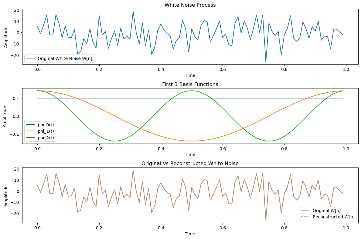
# Visualization
plt.figure(figsize=(12, 8))
# Plot original white noise
plt.subplot(3, 1, 1)
plt.plot(time, W, label="Original White Noise W[n]")
plt.xlabel("Time")
plt.ylabel("Amplitude")
plt.title("White Noise Process")
plt.legend()
# Plot first few basis functions
plt.subplot(3, 1, 2)
for k in range(3):
plt.plot(time, basis[k, :], label=f"phi_{k}(t)")
plt.xlabel("Time")
plt.ylabel("Amplitude")
plt.title("First 3 Basis Functions")
plt.legend()
# Plot original vs reconstructed
plt.subplot(3, 1, 3)
plt.plot(time, W, label="Original W[n]", alpha=0.7)
plt.plot(time, W_reconstructed, '--', label="Reconstructed W[n]", alpha=0.7)
plt.xlabel("Time")
plt.ylabel("Amplitude")
plt.title("Original vs Reconstructed White Noise")
plt.legend()
plt.tight_layout()
plt.show()
# Compute mean squared error to verify reconstruction
mse = np.mean((W - W_reconstructed)**2)
print(f"Mean Squared Error between original and reconstructed: {mse:.2e}")
First 5 coefficients Z_k: [-10.38465174   2.301302     6.58712585  13.29551733   6.81870197]
Original W[n] (first 5): [ 4.96714153 -1.38264301  6.47688538 15.23029856 -2.34153375]
Reconstructed W[n] (first 5): [ 4.64885039 -1.06435188  6.15859424 15.5485897  -2.65982488]
Mean Squared Error between original and reconstructed: 1.01e-01