Binary Antipodal Signaling#
Binary antipodal signaling is a fundamental modulation scheme in digital communications, particularly well-suited for illustrating optimal detection principles in an AWGN channel. In this scheme, there are two possible transmitted signals:
where \( s(t) \) is a base waveform. These signals are antipodal, meaning they are negatives of each other, lying on opposite sides of the origin in signal space. The prior probabilities of transmitting message 1 (\( s_1(t) \)) and message 2 (\( s_2(t) \)) are \( p \) and \( 1 - p \), respectively, allowing for non-uniform priors.
One-Dimensional Signal Space Representation#
Since the signals are scalar multiples of a single waveform \( s(t) \), the signal space is one-dimensional (\( N = 1 \)). Using an orthonormal basis with a single function \( \phi_1(t) \) (e.g., normalized such that
), the vector representations reduce to scalars:
where
is the signal energy. In binary signaling, this is commonly denoted as \( \mathcal{E}_b \) (bit energy), since each signal corresponds to one bit.
Received Signal Model#
In the vector AWGN channel, the received signal is
where:
\( r \) is a scalar (since \( N = 1 \)).
\( s_m \) is either \( \sqrt{\mathcal{E}_b} \) or \( -\sqrt{\mathcal{E}_b} \), depending on which signal was transmitted.
\( n \sim \mathcal{N}(0, N_0/2) \) is Gaussian noise with variance \( N_0/2 \).
Since the signal space is one-dimensional, the detection problem reduces to determining whether \( r \) is closer to \( \sqrt{\mathcal{E}_b} \) or \( -\sqrt{\mathcal{E}_b} \), leading to a simple threshold-based decision rule, which we will explore next.
MAP Decision Rule#
Applying the general MAP decision region formula for the scalar case:
where the bias term is
Computing \( D_1 \) (Region Where \( \hat{m} = 1 \))
For \( m = 1 \):
\( s_1 = \sqrt{\mathcal{E}_b} \), \( P_1 = p \), \( \mathcal{E}_1 = \mathcal{E}_b \).
The bias term is
\[ \eta_1 = \frac{N_0}{2} \ln p - \frac{1}{2} \mathcal{E}_b. \]
For \( m = 2 \):
\( s_2 = -\sqrt{\mathcal{E}_b} \), \( P_2 = 1 - p \), \( \mathcal{E}_2 = \mathcal{E}_b \).
The bias term is
\[ \eta_2 = \frac{N_0}{2} \ln (1 - p) - \frac{1}{2} \mathcal{E}_b. \]
Solving for the Decision Boundary
The decision region \( D_1 \) is determined by the inequality:
Rearranging:
Solving for \( r \):
Defining the threshold:
we obtain the decision regions:
Threshold-Based Decision Rule
If \( r > r_{\tt th} \), decide message 1 (\( s_1 \)).
If \( r \leq r_{\tt th} \), decide message 2 (\( s_2 \)).
The threshold \( r_{\tt th} \) depends on:
Noise power \( N_0 \), which affects detection uncertainty.
Signal energy \( \mathcal{E}_b \), which determines how distinct the signals are.
Prior probabilities \( p \) and \( 1 - p \), which shift the threshold towards the more likely message.
When \( p = 0.5 \) (equiprobable signals), the threshold simplifies to \( r_{\tt th} = 0 \), meaning detection is purely based on whether \( r \) is positive or negative. If priors are unequal, the threshold shifts toward the more probable signal, reducing errors in favor of the more frequent message.
Error Probability#
The probability of error \( P_e \) is the probability that the detector makes an incorrect decision, averaged over the possible transmitted signals. For a binary system, this is expressed as:
where \( P_m \) is the prior probability of message \( m \), and \( p(r | s_m) \) is the conditional probability density function (PDF) of the received signal given that \( s_m \) was transmitted.
Probability of Error Cases
For message 1 (\( s_1 = \sqrt{\mathcal{E}_b} \), transmitted with probability \( p \)), an error occurs when the received signal falls into decision region \( D_2 \):
For message 2 (\( s_2 = -\sqrt{\mathcal{E}_b} \), transmitted with probability \( 1 - p \)), an error occurs when the received signal falls into decision region \( D_1 \):
Thus, the total probability of error is:
Since the decision regions are defined by the threshold \( r_{\tt th} \):
\( D_1 = (r_{\tt th}, \infty) \)
\( D_2 = (-\infty, r_{\tt th}] \),
we rewrite the integral limits:
Gaussian Distributions of \( r \)
Since the received signal model is:
the conditional PDFs of \( r \) are:
which corresponds to:
Similarly,
which corresponds to:
Error Probability in Terms of Q-Function
The probability of error is given by the tail probabilities of these Gaussian distributions. The integrals become:
Using the Q-function, defined as:
we express these probabilities as:
Final Expression for Error Probability
This expression explicitly shows the dependence of the error probability on the threshold \( r_{\tt th} \), making \( P_e \) sensitive to both signal strength and prior probabilities. The result bridges the Gaussian statistics of noise with the decision process, allowing precise performance evaluation of binary antipodal signaling in an AWGN channel.
Special Cases in Binary Antipodal Signaling#
The threshold expression
reveals important behaviors about the decision regions and error probability in different scenarios.
Effect of Prior Probabilities
1️. As \( p \to 0 \) (Message 1 is very unlikely)
The ratio \( \frac{1 - p}{p} \to \infty \), so
\[ r_{\tt th} \to \infty. \]Region \( D_1 \) shrinks to nothing, and \( D_2 \) covers the entire real line.
The detector always selects message 2 (\( s_2 \)), which aligns with \( P_2 \to 1 \).
2️. As \( p \to 1 \) (Message 1 is very likely)
The ratio \( \frac{1 - p}{p} \to 0 \), so
\[ r_{\tt th} \to -\infty. \]Region \( D_2 \) vanishes, and \( D_1 \) covers the entire real line.
The detector always selects message 1 (\( s_1 \)), consistent with \( P_1 \to 1 \).
3️. When \( p = \frac{1}{2} \) (Equiprobable signals)
The term \( \ln \left( \frac{1 - p}{p} \right) = \ln 1 = 0 \), leading to
\[ r_{\tt th} = 0. \]The decision rule simplifies to:
If \( r > 0 \), choose \( s_1 \).
If \( r \leq 0 \), choose \( s_2 \).
This corresponds to a minimum-distance rule, since the decision is based on whether \( r \) is closer to \( \sqrt{\mathcal{E}_b} \) or \( -\sqrt{\mathcal{E}_b} \). The boundary \( r = 0 \) is the midpoint between the two signals.
Error Probability for \( p = \frac{1}{2} \) (BPSK Case)#
For equiprobable signaling, the probability of error is:
Since \( Q(x) = Q(-x) \) for \( x > 0 \), both terms are equal, simplifying to:
This is the classical bit error probability for binary antipodal signaling (e.g., BPSK). Since each message represents one bit, we have:
We can observe that
As SNR increases, \( P_e \) decreases exponentially, showing that higher energy per bit leads to lower error probability.
This fundamental result applies to BPSK, coherent FSK, and other binary modulation schemes, making it one of the most important performance metrics in digital communications.
Simulation#
Note that:
We must use the actual signal amplitudes \(\pm\sqrt{\mathcal{E}_b}\) inside the Q-function, not \(\sqrt{\text{Eb\_N0\_lin}}\).
In the simulation, the transmitted signals are \(\pm\sqrt{\mathcal{E}_b}\) (with \(\mathcal{E}_b=1\) by default). Hence, the means of the Gaussian distributions are \(\pm 1\), not \(\pm \sqrt{\text{Eb\_N0\_lin}}\).
When \(p \neq 0.5\), an incorrect choice of “mean” in the theoretical formula can cause large mismatches between numerical and theoretical \(P_e\). By reverting to the true means (\(\pm\sqrt{\mathcal{E}_b}\)) in the Q-function arguments, the theoretical and simulated curves will match much better.
import numpy as np
import matplotlib.pyplot as plt
from scipy.special import erfc
# ============================================================================
# 1) UTILITY FUNCTIONS
# ============================================================================
def Q(x):
"""
Q-function = 1 - Φ(x) for the standard normal distribution.
Implementation via erfc().
"""
return 0.5 * erfc(x / np.sqrt(2))
def theoretical_pe_general(Eb_N0_lin, p, r_th, Eb=1.0):
"""
General theoretical probability of error for binary antipodal signaling.
- Eb_N0_lin: linear Eb/N0 (not in dB)
- p: prior probability of sending +√Eb
- r_th: decision threshold
- Eb: bit energy (default = 1)
Signals are ±√Eb; AWGN has variance = N0/2, where N0 = Eb/Eb_N0_lin.
"""
N0 = Eb / Eb_N0_lin
sigma = np.sqrt(N0 / 2)
# Means in received space: +√Eb or -√Eb
mean_plus = np.sqrt(Eb)
mean_minus = -np.sqrt(Eb)
# Probability of error given s1 = +√Eb
# if r <= r_th, it's an error => Q((+√Eb - r_th)/σ)
Pe_s1 = Q((mean_plus - r_th) / sigma)
# Probability of error given s2 = -√Eb
# if r > r_th, it's an error => Q((r_th - (-√Eb))/σ) = Q((r_th + √Eb)/σ)
Pe_s2 = Q((r_th - mean_minus) / sigma)
# Combine with priors
return p * Pe_s1 + (1 - p) * Pe_s2
def theoretical_r_th(N0, Eb, p):
"""
MAP threshold for binary antipodal ±√Eb under AWGN.
- N0: noise spectral density
- Eb: bit energy
- p: prior probability of +√Eb
"""
return (N0 / (4.0 * np.sqrt(Eb))) * np.log((1 - p) / p)
# ============================================================================
# 2) MAIN SIMULATION FUNCTION
# ============================================================================
def simulate_antipodal_signaling(Eb_N0_dB, p=0.3, num_bits=100_000):
"""
Simulate binary antipodal (±√Eb) transmission with AWGN.
- Eb_N0_dB: Eb/N0 in dB
- p: prior probability of sending s1= +√Eb
- num_bits: number of bits
Returns (r, bits, r_th_theo, r_th_num, pe_theo_thr, pe_min_err):
r : received samples
bits : transmitted bits (0 or 1)
r_th_theo : theoretical MAP threshold
r_th_num : threshold found by brute force (minimize observed error)
pe_theo_thr : observed BER using r_th_theo
pe_min_err : observed BER using the best threshold
"""
# Convert Eb/N0 to linear scale
Eb_N0_lin = 10 ** (Eb_N0_dB / 10.0)
# Normalized bit energy
Eb = 1.0
N0 = Eb / Eb_N0_lin
# Noise standard deviation
sigma = np.sqrt(N0 / 2)
# Antipodal signals = ±√Eb
s1 = +np.sqrt(Eb)
s2 = -np.sqrt(Eb)
# Generate bits with prior p
bits = (np.random.rand(num_bits) < p).astype(int)
transmitted = np.where(bits == 1, s1, s2)
# Pass through AWGN
noise = np.random.normal(0, sigma, num_bits)
r = transmitted + noise
# Theoretical threshold
# For p=0.5, the threshold is 0; else use formula
if abs(p - 0.5) < 1e-12:
r_th_theo = 0.0
else:
r_th_theo = theoretical_r_th(N0, Eb, p)
# Observed BER using r_th_theo
decisions_theo = (r > r_th_theo).astype(int)
pe_theo_thr = np.mean(decisions_theo != bits)
# Brute-force search for best threshold to minimize error
# (Here we search from -1.5 to +1.5 in small steps; adjust as needed)
r_th_candidates = np.linspace(-1.5, 1.5, 301)
best_thr = None
min_errors = num_bits + 1
for thr in r_th_candidates:
decisions = (r > thr).astype(int)
errors = np.sum(bits != decisions)
if errors < min_errors:
min_errors = errors
best_thr = thr
pe_min_err = min_errors / num_bits
r_th_numerical = best_thr
return r, bits, r_th_theo, r_th_numerical, pe_theo_thr, pe_min_err
# ============================================================================
# 3) SCRIPT: RUN SIMS, PLOT BER, THRESHOLDS, DECISION REGIONS
# ============================================================================
def main():
# You can change p as desired to see how threshold shifts with prior imbalance
p = 0.9
Eb_N0_dB_range = np.arange(0, 11, 1)
num_bits = 200_000 # Increase for smoother curves
# Arrays to store results
theoretical_pe_vals = [] # from formula using r_th_theo
numerical_pe_theo_thr = [] # simulation using r_th_theo
numerical_pe_min_err = [] # simulation using best threshold
theoretical_r_th_vals = []
numerical_r_th_vals = []
# Variables for storing the data at Eb/N0=5 dB for the decision-region plot
last_r = None
last_bits = None
last_r_th_theo = None
# 3.1) Main loop over Eb/N0
for Eb_N0_dB in Eb_N0_dB_range:
(r, bits, r_th_theo, r_th_num, pe_theo_thr, pe_min_err) = \
simulate_antipodal_signaling(Eb_N0_dB, p, num_bits)
# Compute theoretical P(e) from the closed-form formula, using r_th_theo
Eb_N0_lin = 10 ** (Eb_N0_dB / 10.0)
pe_theo = theoretical_pe_general(Eb_N0_lin, p, r_th_theo, Eb=1.0)
theoretical_pe_vals.append(pe_theo)
numerical_pe_theo_thr.append(pe_theo_thr)
numerical_pe_min_err.append(pe_min_err)
theoretical_r_th_vals.append(r_th_theo)
numerical_r_th_vals.append(r_th_num)
# Save data for plotting decision region if Eb/N0=5
if Eb_N0_dB == 5:
last_r = r
last_bits = bits
last_r_th_theo = r_th_theo
# 3.2) Plot: BER vs. Eb/N0
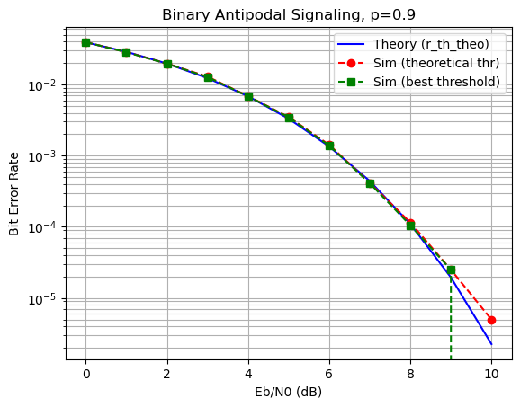
plt.figure()
plt.semilogy(Eb_N0_dB_range, theoretical_pe_vals, 'b-', label='Theory (r_th_theo)')
plt.semilogy(Eb_N0_dB_range, numerical_pe_theo_thr, 'ro--',label='Sim (theoretical thr)')
plt.semilogy(Eb_N0_dB_range, numerical_pe_min_err, 'gs--',label='Sim (best threshold)')
plt.grid(True, which='both')
plt.xlabel('Eb/N0 (dB)')
plt.ylabel('Bit Error Rate')
plt.title(f'Binary Antipodal Signaling, p={p}')
plt.legend()
plt.show()
# 3.3) Plot: threshold vs. Eb/N0
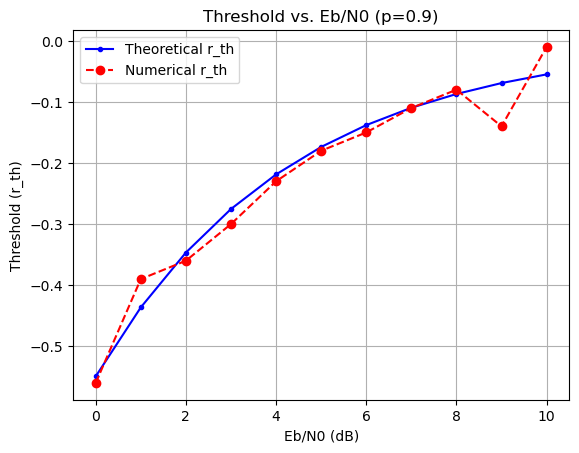
plt.figure()
plt.plot(Eb_N0_dB_range, theoretical_r_th_vals, 'b.-', label='Theoretical r_th')
plt.plot(Eb_N0_dB_range, numerical_r_th_vals, 'ro--', label='Numerical r_th')
plt.grid(True)
plt.xlabel('Eb/N0 (dB)')
plt.ylabel('Threshold (r_th)')
plt.title(f'Threshold vs. Eb/N0 (p={p})')
plt.legend()
plt.show()
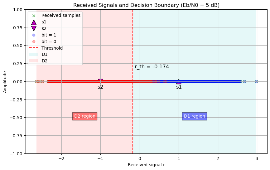
# 3.4) Decision Regions at Eb/N0=5 dB
if last_r is not None:
plt.figure(figsize=(10, 6))
# Plot all received samples (green x's at y=0)
plt.scatter(
last_r,
np.zeros_like(last_r),
c='g',
marker='x',
label='Received samples',
alpha=0.5
)
# Plot nominal signal points: s1 = +1, s2 = -1
plt.scatter(
1.0, 0,
s=133,
c='m',
marker='^',
edgecolors='k',
label='s1'
)
plt.text(1.0, -0.1, 's1', fontsize=12, ha='center')
plt.scatter(
-1.0, 0,
s=133,
c='m',
marker='v',
edgecolors='k',
label='s2'
)
plt.text(-1.0, -0.1, 's2', fontsize=12, ha='center')
# Color-code received samples by the transmitted bit
plt.scatter(
last_r[last_bits == 1],
np.zeros((last_bits == 1).sum()),
c='b',
marker='o',
alpha=0.3,
label='bit = 1'
)
plt.scatter(
last_r[last_bits == 0],
np.zeros((last_bits == 0).sum()),
c='r',
marker='o',
alpha=0.3,
label='bit = 0'
)
# Draw the theoretical decision threshold
plt.axvline(
x=last_r_th_theo,
color='r',
linestyle='--',
label='Threshold'
)
plt.text(
last_r_th_theo + 0.05,
0.2,
f'r_th = {last_r_th_theo:.3f}',
ha='left',
va='center',
fontsize=12
)
# Shade decision regions
y_lim = [-1, 1]
r_min, r_max = min(last_r), max(last_r)
# D1 region = {r > threshold}
plt.fill(
[last_r_th_theo, r_max, r_max, last_r_th_theo],
[y_lim[0], y_lim[0], y_lim[1], y_lim[1]],
facecolor='c',
alpha=0.1,
edgecolor='none',
label='D1'
)
# D2 region = {r <= threshold}
plt.fill(
[r_min, last_r_th_theo, last_r_th_theo, r_min],
[y_lim[0], y_lim[0], y_lim[1], y_lim[1]],
facecolor='r',
alpha=0.1,
edgecolor='none',
label='D2'
)
# Labels for each region
plt.text(
0.5 * (last_r_th_theo + r_max),
-0.5,
'D1 region',
ha='center',
bbox=dict(facecolor='blue', alpha=0.5),
color='white'
)
plt.text(
0.5 * (r_min + last_r_th_theo),
-0.5,
'D2 region',
ha='center',
bbox=dict(facecolor='red', alpha=0.5),
color='white'
)
plt.xlabel('Received signal r')
plt.ylabel('Amplitude')
plt.title('Received Signals and Decision Boundary (Eb/N0 = 5 dB)')
plt.ylim(y_lim)
plt.legend(loc='upper left')
plt.grid(True)
plt.show()
else:
print("[INFO] Eb/N0 = 5 dB data not found or p != 0.5 loop never triggered that condition.")
# ============================================================================
# 4) RUN IT
# ============================================================================
if __name__ == "__main__":
main()