Minimum Variance Estimaties#
The objective in estimation is to find an estimate \(\hat{\boldsymbol{\alpha}}\) that is close to the true parameter \(\alpha\).
This closeness is desired even if the estimator is biased.
Variance as a Measure of The Closeness
For an unbiased estimator, variance (\( V\{\hat{\boldsymbol{\alpha}}\} = E\{(\hat{\boldsymbol{\alpha}} - \alpha)^2\} \)) measures the variability of the estimator around the true parameter.
This variance is equivalent to the mean-squared error between the estimate and the true parameter value.
Choosing Between Estimators:
When comparing two unbiased estimators, \(\hat{\boldsymbol{\alpha}}_1\) and \(\hat{\boldsymbol{\alpha}}_2\), with variances \(V\{\hat{\boldsymbol{\alpha}}_1\}\) and \(V\{\hat{\boldsymbol{\alpha}}_2\}\), it is logical to choose the estimator with the smaller variance, i.e., \(\hat{\boldsymbol{\alpha}}_2\) if \(V\{\hat{\boldsymbol{\alpha}}_2\} \leq V\{\hat{\boldsymbol{\alpha}}_1\}\).
While unbiasedness is a desirable property, it does not guarantee a realizable or optimal estimate.
Sometimes biased estimators can achieve lower mean-squared error compared to unbiased ones.
Indeed, there exist biased estimators with smaller mean-squared error compared to unbiased estimators, and these biased estimators can become asymptotically unbiased.
Such biased estimators can be advantageous despite their bias.
Chebyshev’s Inequality#
Chebyshev’s inequality is a fundamental result in probability theory that provides an upper bound on the probability that a random variable deviates from its mean by more than a certain amount.
The theorem is stated as:
Suppose that \( \mathbf{x} \) is a random variable with mean \( \mu_{\mathbf{x}} \) and variance \( \sigma_{\mathbf{x}}^2 \). The probability that the random variable \( {\mathbf{x}} \) takes on a value that is removed from the mean by more than \( x_0 \) is given by:
Apllying the Chebyshev’s inequality into estimation theorey, we have that, for an estimate \(\hat{\boldsymbol{\alpha}}\) (where the bold symbol indicates that it is a random variable) of a true parameter \(\alpha\) (the normal symbol indicating a specific value), Chebyshev’s inequality can be expressed as:
Here:
\(\Pr\left(|\hat{\boldsymbol{\alpha}} - \alpha| > \epsilon\right)\) is the probability that the estimator \(\hat{\boldsymbol{\alpha}}\) deviates from the true value \(\alpha\) by more than a threshold \(\epsilon\).
\(V(\hat{\boldsymbol{\alpha}})\) represents the variance of the estimator \(\hat{\boldsymbol{\alpha}}\), defined as:
\[ V(\hat{\boldsymbol{\alpha}}) = E\left\{(\hat{\boldsymbol{\alpha}} - \alpha)^2\right\} \]This is the expected value of the squared difference between the estimator and the true value, essentially measuring the spread or dispersion of the estimator around the true value.
The inequality shows that the probability of the estimator being far from the true value decreases as the variance of the estimator decreases.
Therefore, to minimize the probability of large errors, we desire an estimator with a small variance.
Cramér-Rao Lower Bound#
In statistical estimation theory, the Cramér-Rao inequality provides a lower bound on the variance of any unbiased estimator of a parameter.
It tells us how good an estimator can be in terms of its variance.
Specifically, for an unbiased estimator \(\hat{\boldsymbol{\alpha}}\), the variance \(V(\hat{\boldsymbol{\alpha}})\) must satisfy the following inequality:
where:
\(p(\vec{y};\alpha)\) is the likelihood function, representing the probability of observing the data \(\vec{\mathbf{y}}\) given the parameter \(\alpha\).
\(\frac{\partial^2}{\partial\alpha^2}\ln p(\vec{y};\alpha)\) is the second derivative of the log-likelihood function with respect to the parameter \(\alpha\), which measures the curvature of the likelihood function.
A higher curvature implies that small changes in \(\alpha\) lead to significant changes in the likelihood, meaning the parameter is estimated with high precision.
The expected value of this curvature (in the denominator) quantifies the amount of information about \(\alpha\) that is contained in the data \(\vec{\mathbf{y}}\).
The inverse of this quantity represents the smallest possible variance that any unbiased estimator can achieve—the Cramér-Rao lower bound.
Fisher Information \(F(\alpha)\)
The lower bound of \(V\{\hat{\boldsymbol{\alpha}}\}\) can be expressed as
where \( p(y_1, \ldots, y_m; \alpha) \) is the probability density function of the observations.
The denominator of the inequality is known as the Fisher information, denoted as \( F(\alpha) \), i.e.,
Thus, we have
A larger value of the Fisher information \( F(\alpha) \) implies that more information is known about the estimate, leading to a smaller variance.
Most Efficient Estimate#
An estimate \(\hat{\boldsymbol{\alpha}}\) that achieves the Cramér-Rao lower bound is considered the most efficient estimate because it has the minimum possible variance among all unbiased estimators.
In practice, this means that the estimate is as close as possible to the true value \(\alpha\) given the available data, minimizing the spread of the estimator’s possible values around the true parameter.
If an estimate achieves this bound, it is optimal in the sense of having the smallest variance, thus being the most reliable and precise estimator given the data.
Example: The Most Efficient Estimator of the True Mean#
Problem
In this exmaple (based on [B2, Ex 10.3], we find the most efficient estimator of the true mean given the data that is the independent, normally distributed, random variables \( \mathbf{y}_1, \dots, \mathbf{y}_m \) with true mean \( \mu \) and variance \( \sigma^2 \).
Solution
The sample mean \( \bar{\mathbf{y}} \) is an efficient estimate of the true mean \( \mu \), as shown in the following argument.
Proof
The sample mean is unbiased (as shown in previous examples) and its variance is
The right-hand side of the Cramér-Rao inequality, i.e., \( F^{-1}(\mu) \), is derived as
Thus, we have
Thus, we have
Therefore, we have
The inequality is satisfied with equality in this case.
the sample mean \( \bar{\mathbf{y}} \) is a most efficient estimate for the true mean \( \mu \) of the distribution.
Discussion. Estimator vs Estimate
The term sample mean \( \bar{\mathbf{y}} \) can refer to both the estimator (the rule, the formula, or the method) and the estimate (the obtained value from the data). This dual usage is common in statistical discussions where the method and the result are closely related.
import numpy as np
import matplotlib.pyplot as plt

# Parameters for the normal distribution
mu = 5  # true mean
sigma = 2  # true standard deviation
m = 50  # sample size
n_samples = 1000  # number of samples to draw

# Generate multiple samples and compute sample means
sample_means = np.zeros(n_samples)
for i in range(n_samples):
    sample = np.random.normal(mu, sigma, m)
    sample_means[i] = np.mean(sample)

# Empirical variance of the sample means
empirical_variance = np.var(sample_means, ddof=1)

# Theoretical Cramér-Rao lower bound for the variance of the sample mean
theoretical_variance = sigma**2 / m

# Display the results
print(f"Empirical Variance of Sample Means: {empirical_variance:.4f}")
print(f"Theoretical Minimum Variance (Cramér-Rao Bound): {theoretical_variance:.4f}")

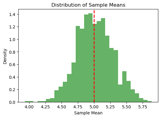
# Plotting the distribution of the sample means
plt.figure(figsize=(6, 4))
plt.hist(sample_means, bins=30, density=True, alpha=0.6, color='g')
plt.axvline(mu, color='red', linestyle='dashed', linewidth=2)
plt.title("Distribution of Sample Means")
plt.xlabel("Sample Mean")
plt.ylabel("Density")
plt.show()
Empirical Variance of Sample Means: 0.0797
Theoretical Minimum Variance (Cramér-Rao Bound): 0.0800

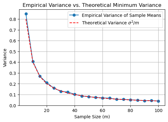
Variance of the sample mean as a function of the number of data samples#
import numpy as np
import matplotlib.pyplot as plt

# Parameters for the normal distribution
mu = 5  # true mean
sigma = 2  # true standard deviation
n_samples = 1000  # number of samples to draw for each m
sample_sizes = np.arange(5, 101, 5)  # different sample sizes

# Initialize arrays to store variances
empirical_variances = []
theoretical_variances = []

# Calculate variances for different sample sizes
for m in sample_sizes:
    sample_means = np.zeros(n_samples)
    for i in range(n_samples):
        sample = np.random.normal(mu, sigma, m)
        sample_means[i] = np.mean(sample)

    # Empirical variance of the sample means
    empirical_variance = np.var(sample_means, ddof=1)
    empirical_variances.append(empirical_variance)

    # Theoretical minimum variance (Cramér-Rao bound)
    theoretical_variance = sigma**2 / m
    theoretical_variances.append(theoretical_variance)

# Plotting the results
plt.figure(figsize=(6, 4))
plt.plot(sample_sizes, empirical_variances, 'o-', label="Empirical Variance of Sample Means")
plt.plot(sample_sizes, theoretical_variances, 'r--', label=r"Theoretical Variance $\sigma^2 / m$")
plt.xlabel("Sample Size (m)")
plt.ylabel("Variance")
plt.title("Empirical Variance vs. Theoretical Minimum Variance")
plt.legend()
plt.grid(True)
plt.show()

Example: Comparing Different Estimates#
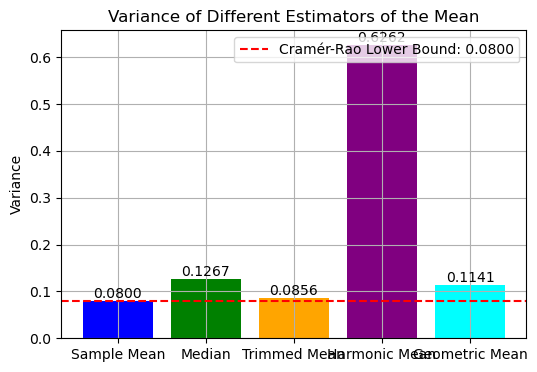
We consider: sample mean, median, trimmed mean, harmonic mean, or geometric mean as estimators of the true mean.
Median
The median is the value separating the higher half from the lower half of the sample. For a sample of size \( m \):
If \( m \) is odd, the median is the middle value when the sample is sorted.
If \( m \) is even, the median is the average of the two middle values when the sample is sorted.
Mathematically:
where \( \mathbf{y}_{(i)} \) denotes the \( i \)-th smallest value in the sorted sample.
Trimmed Mean
The trimmed mean is an average computed after removing a specified percentage of the smallest and largest values from the sample. For a \( \lambda\%- \) trimmed mean:
where:
\( \mathbf{y}_{(1)} \leq \mathbf{y}_{(2)} \leq \dots \leq \mathbf{y}_{(m)} \) is the sorted sample.
\( k = \left\lfloor \frac{\lambda \times m}{100} \right\rfloor \) is the number of values trimmed from each end of the sample.
Harmonic Mean
The harmonic mean is the reciprocal of the arithmetic mean of the reciprocals of the sample values. It is defined as:
where:
\( \mathbf{y}_i > 0 \) for all \( i \) (the harmonic mean is only defined for positive values).
\( m \) is the number of observations in the sample.
Geometric Mean
The geometric mean is the \( m \)-th root of the product of the sample values. It is defined as:
where:
\( \mathbf{y}_i > 0 \) for all \( i \) (the geometric mean is only defined for positive values).
\( m \) is the number of observations in the sample.
import numpy as np
import matplotlib.pyplot as plt
from scipy.stats import hmean, gmean

# Parameters for the normal distribution
mu = 5  # true mean
sigma = 2  # true standard deviation
m = 50  # sample size
n_samples = 1000  # number of samples to draw

# Initialize arrays to store the estimators
sample_means = np.zeros(n_samples)
medians = np.zeros(n_samples)
trimmed_means = np.zeros(n_samples)
harmonic_means = []
geometric_means = []

# Generate samples and compute the estimators
for i in range(n_samples):
    sample = np.random.normal(mu, sigma, m)

    # Compute the estimators that don't require positive-only values
    sample_means[i] = np.mean(sample)
    medians[i] = np.median(sample)
    trimmed_means[i] = np.mean(np.sort(sample)[int(0.1*m):int(0.9*m)])  # 10% trimmed mean

    # Check for positive values before calculating the harmonic and geometric means
    if np.all(sample > 0):
        harmonic_means.append(hmean(sample))
        geometric_means.append(gmean(sample))

# Convert harmonic_means and geometric_means to numpy arrays
harmonic_means = np.array(harmonic_means)
geometric_means = np.array(geometric_means)

# Compute the empirical variances of the estimators
variance_sample_mean = np.var(sample_means, ddof=1)
variance_median = np.var(medians, ddof=1)
variance_trimmed_mean = np.var(trimmed_means, ddof=1)
variance_harmonic_mean = np.var(harmonic_means, ddof=1) if len(harmonic_means) > 0 else np.nan
variance_geometric_mean = np.var(geometric_means, ddof=1) if len(geometric_means) > 0 else np.nan

# Theoretical variance of the sample mean (Cramér-Rao lower bound)
theoretical_variance = sigma**2 / m

# Print the results
print(f"Empirical Variance of Sample Mean: {variance_sample_mean:.4f}")
print(f"Empirical Variance of Median: {variance_median:.4f}")
print(f"Empirical Variance of Trimmed Mean: {variance_trimmed_mean:.4f}")
print(f"Empirical Variance of Harmonic Mean: {variance_harmonic_mean:.4f}")
print(f"Empirical Variance of Geometric Mean: {variance_geometric_mean:.4f}")
print(f"Theoretical Minimum Variance (Cramér-Rao Bound): {theoretical_variance:.4f}")

# Visualizing the variances
estimators = ['Sample Mean', 'Median', 'Trimmed Mean', 'Harmonic Mean', 'Geometric Mean']
variances = [variance_sample_mean, variance_median, variance_trimmed_mean, variance_harmonic_mean, variance_geometric_mean]

plt.figure(figsize=(6, 4))
bars = plt.bar(estimators, variances, color=['blue', 'green', 'orange', 'purple', 'cyan'])
plt.axhline(theoretical_variance, color='red', linestyle='--', label=f"Cramér-Rao Lower Bound: {theoretical_variance:.4f}")

# Add the variance value on top of each bar
for bar, variance in zip(bars, variances):
    yval = bar.get_height()
    plt.text(bar.get_x() + bar.get_width()/2, yval, f'{variance:.4f}', ha='center', va='bottom')

plt.ylabel("Variance")
plt.title("Variance of Different Estimators of the Mean")
plt.legend()
plt.grid(True)
plt.show()
Empirical Variance of Sample Mean: 0.0800
Empirical Variance of Median: 0.1267
Empirical Variance of Trimmed Mean: 0.0856
Empirical Variance of Harmonic Mean: 0.6262
Empirical Variance of Geometric Mean: 0.1141
Theoretical Minimum Variance (Cramér-Rao Bound): 0.0800

Discussion. Numerical Error in Simulation
The empirical variance of the sample mean sometimes being slightly lower than the theoretical Cramér-Rao bound, e.g., Empirical Variance of Sample Mean = \(0.0795\) while Theoretical Minimum Variance (Cramér-Rao Bound) = \(0.0800\).
This can occur due to the nature of statistical estimation and the finite number of samples used to compute the empirical variance.
The small difference between the empirical variance and the Cramér-Rao bound is normal and expected in practical simulations.
