Minimum Mean Squared Error (MMSE) Estimation#
In Bayesian estimation, when we aim to minimize the mean squared error (MSE) between the true parameter \(\alpha\) and our estimate \(\hat{\alpha}\), we use the squared-error cost function.
The conditional cost function \(C_{\text{MSE}}(\hat{\alpha}|\vec{y})\) represents the expected squared error given the observations \(\vec{y}\) and is defined as:
Note that this is not merely a definition; it’s an equation representing how the cost varies with \(\hat{\alpha}\).
Our goal is to find the estimate \(\hat{\alpha}\) that minimizes this conditional cost function.
To achieve this, from the optimization theory:
we treat \(C_{\text{MSE}}(\hat{\alpha}|\vec{y})\) as a function of \(\hat{\alpha}\)
perform optimization by taking its derivative with respect to \(\hat{\alpha}\),
setting the derivative equal to zero,
solving for \(\hat{\alpha}\).
Mathematical Description#
First, differentiating \(C_{\text{MSE}}(\hat{\alpha}|\vec{y})\) with respect to \(\hat{\alpha}\), we have
On the RHS, calculating the derivative inside the integral, we have
Thus, we obtain
Next, setting the derivative equal to zero to find the minimum:
Simplifying (dividing both sides by \(-2\)):
Next, expanding the integral:
Recognizing that:
\(\int_{-\infty}^{\infty} p(\alpha|\vec{y})\, d\alpha = 1\) (since \(p(\alpha|\vec{y})\) is a probability density function)
\(\hat{\alpha}\) does not depend on \(\alpha\) and can be taken out of the integral
We get:
We observe that the second derivative of \(C_{\text{MSE}}(\hat{\alpha}|\vec{y})\) with respect to \(\hat{\alpha}\) is positive:
This confirms that the critical point found is indeed a minimum.
The right-hand side of the equation is the expected value (mean) of RV \(\boldsymbol{\alpha}\) given \(\vec{y}\), denoted as \(E\{\boldsymbol{\alpha}|\vec{y}\}\), we have
Alternative Form of MSE Estimator#
An alternative form of \(\hat{\boldsymbol{\alpha}}_{\text{MMSE}}\) can be obtained by using the identities
and
resulting in
This form requires the pdfs \(p(\vec{y}|\alpha)\) and \(p(\alpha)\) instead of the a posteriori pdf \(p(\alpha|\vec{y})\) to compute \(\hat{\alpha}_{\text{MSE}}\) and is often simpler to evaluate.
Discussion: An optimal estimate for a more general class of cost functions#
In Bayesian estimation, the conditional mean \( E\{\alpha | \vec{y}\} \) is well-known for minimizing the mean squared error (MSE) cost function.
However, its optimality extends to a broader class of cost functions under certain conditions.
First Case: Convex and Symmetric Cost Functions
Convexity and Symmetry: If the cost function \( C(\alpha_e) \) is convex and symmetric with respect to the estimation error \( \boldsymbol{\alpha}_e = \boldsymbol{\alpha} - \hat{\boldsymbol{\alpha}} \), meaning \(C(\alpha,\hat{\alpha}) = C(\alpha_e)\), and \( C(\alpha_e) = C(-\alpha_e) \), then the conditional mean remains the optimal estimator.
Convexity ensures that the cost increases at an increasing rate as the error grows, penalizing larger errors more severely.
Symmetry means that overestimation and underestimation are penalized equally.
Optimality of Conditional Mean: Under these conditions, minimizing the expected cost leads to the conditional mean because it balances the errors due to the symmetric nature of both the cost function and the posterior distribution.
Second Case: Symmetric, Nondecreasing Cost Functions with Specific Posterior Properties
Symmetric and Nondecreasing Cost Function: The cost function \( C(\alpha_e) \) is symmetric (\( C(\alpha_e) = C(-\alpha_e) \)) and nondecreasing for \( \alpha_e \geq 0 \), i.e., \(C(\alpha_{e_2}) > C(\alpha_{e_1})\), for \(\alpha_{e_2} \geq \alpha_{e_1} \geq 0\). This means that the cost does not decrease as the magnitude of the error increases
Posterior PDF Conditions:
The posterior probability density function \( p(\alpha | \vec{y}) \) is symmetric about its mean and unimodal (has a single peak).
It satisfies the condition:
\[ \lim_{\alpha_e \to \infty} C(\alpha_e) p(\alpha_e | \vec{y}) = 0 \]This condition ensures that the product of the cost and the tail of the posterior distribution diminishes to zero, making the expected cost finite and well-defined.
Optimality of Conditional Mean: Under these circumstances, the conditional mean minimizes the expected cost because:
The symmetry of \( p(\alpha | \vec{y}) \) ensures that the mean is at the center of the distribution.
The nondecreasing nature of \( C(\alpha_e) \) penalizes larger errors more heavily.
The diminishing product, i.e., \(\to 0\) as \(m \to \infty\), guarantees that extreme errors contribute negligibly to the expected cost.
Example C3.7: MMSE Estimator (Bayes estimator that minimize the MSE cost function)#
Problem Statement
In this example, based on [B2, Ex 10.7], we want to find the estimate \(\hat{\boldsymbol{\mu}}\) of the unknown random mean \(\boldsymbol{\mu}\), using the set of observations \(\mathbf{y}_1, \ldots, \mathbf{y}_m\).
Assume further that the observations are statistically independent, normal random variables, each with unknown mean \(\boldsymbol{\mu}\) and known variance \(\sigma^2\).
The conditional pdf \(p(\vec{y}|\mu)\) is then
Next, assume that the a priori pdf \(p(\mu)\) is normal with mean \(m_1\) and variance \(\beta^2\), i.e.,
Note that the prior \( p(\mu) \) represents our knowledge about \(\mu\) before observing any data.
Discussion. Conditional i.i.d.#
In the example, the mean \(\boldsymbol{\mu}\) is treated as a random variable with a prior distribution \( p(\mu) \), and yet the observations \( \mathbf{y}_1, \mathbf{y}_2, \ldots, \mathbf{y}_m \) are considered independent and identically distributed (i.i.d.).
This might seem contradictory at first, but it makes sense within the Bayesian framework due to the concept of conditional independence.
Conditional Independence Given \(\mu\)
The observations \( \mathbf{y}_i \) are conditionally independent given the parameter \(\mu\) (a realization of \(\boldsymbol{\mu}\)).
This means that once the value of \(\mu\) is specified, the observations are independent of each other.
\[ p(y_1, y_2, \ldots, y_m | \mu) = \prod_{i=1}^m p(y_i | \mu) \]Each \( y_i \) (a relization of RV \(\mathbf{y}_i\)) is generated from the same distribution \( \mathcal{N}(\mu, \sigma^2) \), making them identically distributed given \(\mu\).
Unconditional Dependence Due to Random \(\mu\)
Dependence through \(\mu\): Since \(\boldsymbol{\mu}\) is a random variable, it introduces dependence among the observations when we consider their joint distribution without conditioning on \(\boldsymbol{\mu}\).
Joint Distribution Without Conditioning:
\[ p(y_1, y_2, \ldots, y_m) = \int_{-\infty}^\infty \left( \prod_{i=1}^m p(y_i | \mu) \right) p(\mu) d\mu \]This integral over \(\mu\) mixes the observations together, reflecting their dependence.
Why We Consider i.i.d. in the Likelihood Function:
Conditional Likelihood: In Bayesian estimation, we work with the likelihood function \( p(\vec{y} | \mu) \), which treats the observations as independent given \(\mu\).
This conditional independence allows us to factor the likelihood and simplify the estimation process.
Finding the MMMSE Estimate#
In the sequence of this chapter, note that the terms MMSE Estimate and MMMSE Estimate are interchangeable.
Recall that the MSE estimate is defined as
Thus, we need to find the a posteriori \(p(\alpha|\vec{y})\).
From
and
the a posteriori pdf can be obtained as
where
and
and
See the Appendix for the derivation.
Again, \(\hat{\boldsymbol{\alpha}}_{\text{MMSE}} = \int_{-\infty}^{\infty} \alpha\, p(\alpha|\vec{y})\, d\alpha\), the Bayes estimate can now be obtained as
It follows that the random estimate \(\hat{\mu}_{\text{MMSE}}\) can be written as
Simulation#
Objective:
Simulate the Bayesian estimation of an unknown random mean \( \boldsymbol{\mu} \) using observed data \( \mathbf{y}_1, \mathbf{y}_2, \ldots, \mathbf{y}_m \).
The true mean \( \boldsymbol{\mu}_{\text{true}} \) is a random variable drawn from the prior distribution \( p(\mu) \), which is normal with a known, fixed mean \( m_1 \) and a known, fixed variance \( \beta^2 \).
Each observation \( \mathbf{y}_k \) is then generated from a normal distribution with mean \( \mu_{\text{true}} \) (a realization of \( \boldsymbol{\mu}_{\text{true}} \)) and known variance \( \sigma^2 \).
We aim to compute the Bayesian MMSE estimator \( \hat{\mu}_{\text{MMSE}} \) and compare it with the true mean \( \mu_{\text{true}} \).
Simulation Steps:
Set the Parameters:
Prior Mean (\( m_1 \)): Mean of the prior distribution.
Prior Variance (\( \beta^2 \)): Variance of the prior distribution.
Observation Variance (\( \sigma^2 \)): Known variance of the observations.
Number of Observations (\( m \)): The number of data points.
Number of Simulations: To assess estimator performance over multiple trials.
Generate the True Mean (\( \mu_{\text{true}} \)):
Sample \( \mu_{\text{true}} \) from the prior distribution \( \mathcal{N}(m_1, \beta^2) \).
Generate Observations:
For \( k = 1 \) to \( m \), sample \( y_k \) from \( \mathcal{N}(\mu_{\text{true}}, \sigma^2) \).
Compute the Sample Mean (\( \bar{y} \)):
Calculate \( \bar{y} = \frac{1}{m} \sum_{k=1}^m y_k \).
Compute the Bayesian MMSE Estimator (\( \hat{\mu}_{\text{MMSE}} \)):
Use the formula: $\( \hat{\mu}_{\text{MMSE}} = \frac{\beta^2 \bar{y} + m_1 \sigma^2 / m}{\beta^2 + \sigma^2 / m} \)$
Compare \( \mu_{\text{true}} \) and \( \hat{\mu}_{\text{MMSE}} \):
Calculate the estimation error \( \hat{\mu}_{\text{MMSE}} - \mu_{\text{true}} \).
Repeat the simulation multiple times to evaluate the estimator’s performance.
import numpy as np
import matplotlib.pyplot as plt

# Set random seed for reproducibility
np.random.seed(42)

# Parameters
m1 = 0.0            # Prior mean
beta2 = 9.0         # Prior variance (β^2)
beta = np.sqrt(beta2)
sigma2 = 4.0        # Known variance of observations (σ^2)
sigma = np.sqrt(sigma2)
m = 10              # Number of observations
num_simulations = 1000  # Number of simulations

# Arrays to store estimates and true means
mu_true_values = []
mu_estimates_mmse = []
mu_estimates_sample_mean = []

for _ in range(num_simulations):
    # Step 2: Generate the true mean mu_true from the prior
    mu_true = np.random.normal(m1, beta)
    mu_true_values.append(mu_true)

    # Step 3: Generate observed data y_k ~ N(mu_true, sigma^2)
    y = np.random.normal(mu_true, sigma, m)

    # Step 4: Compute the sample mean
    y_bar = np.mean(y)

    # Step 5: Compute the Bayesian MMSE estimator
    numerator = beta2 * y_bar + m1 * sigma2 / m
    denominator = beta2 + sigma2 / m
    mu_hat_mmse = numerator / denominator

    # Store the estimates
    mu_estimates_mmse.append(mu_hat_mmse)
    mu_estimates_sample_mean.append(y_bar)

# Convert lists to arrays
mu_true_values = np.array(mu_true_values)
mu_estimates_mmse = np.array(mu_estimates_mmse)
mu_estimates_sample_mean = np.array(mu_estimates_sample_mean)

# Step 6: Compute the Mean Squared Errors
mse_bayes_mmse = np.mean((mu_estimates_mmse - mu_true_values) ** 2)
mse_sample_mean = np.mean((mu_estimates_sample_mean - mu_true_values) ** 2)

print(f"Bayesian MMSE Estimator Mean Squared Error: {mse_bayes_mmse:.4f}")
print(f"Sample Mean Estimator Mean Squared Error: {mse_sample_mean:.4f}")

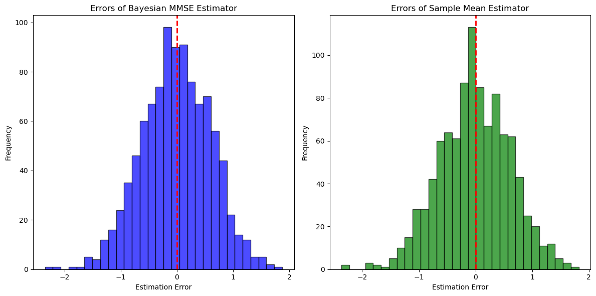
# Plotting the estimation errors
plt.figure(figsize=(12, 6))

# Histogram of errors for Bayesian MMSE estimator
plt.subplot(1, 2, 1)
errors_bayes_mmse = mu_estimates_mmse - mu_true_values
plt.hist(errors_bayes_mmse, bins=30, alpha=0.7, color='blue', edgecolor='black')
plt.axvline(0, color='red', linestyle='dashed', linewidth=2)
plt.title('Errors of Bayesian MMSE Estimator')
plt.xlabel('Estimation Error')
plt.ylabel('Frequency')

# Histogram of errors for Sample Mean estimator
plt.subplot(1, 2, 2)
errors_sample_mean = mu_estimates_sample_mean - mu_true_values
plt.hist(errors_sample_mean, bins=30, alpha=0.7, color='green', edgecolor='black')
plt.axvline(0, color='red', linestyle='dashed', linewidth=2)
plt.title('Errors of Sample Mean Estimator')
plt.xlabel('Estimation Error')
plt.ylabel('Frequency')

plt.tight_layout()
plt.show()
Bayesian MMSE Estimator Mean Squared Error: 0.3754
Sample Mean Estimator Mean Squared Error: 0.3826

import numpy as np
import matplotlib.pyplot as plt

# Set random seed for reproducibility
np.random.seed(42)

# Parameters
m1 = 0.0            # Prior mean
beta2 = 9.0         # Prior variance (β^2)
beta = np.sqrt(beta2)
sigma2 = 4.0        # Known variance of observations (σ^2)
sigma = np.sqrt(sigma2)
m_values = [1, 2, 5, 10, 20, 50, 100, 1000]  # Different values of m
num_simulations = 1000  # Number of simulations for each m

# Arrays to store results
mean_abs_errors = []
std_abs_errors = []
mse_errors = []

for m in m_values:
    estimation_errors = []

    for _ in range(num_simulations):
        # Step 2: Generate the true mean mu_true from the prior
        mu_true = np.random.normal(m1, beta)

        # Step 3: Generate observed data y_k ~ N(mu_true, sigma^2)
        y = np.random.normal(mu_true, sigma, m)

        # Step 4: Compute the sample mean
        y_bar = np.mean(y)

        # Step 5: Compute the Bayesian MMSE estimator
        numerator = beta2 * y_bar + m1 * sigma2 / m
        denominator = beta2 + sigma2 / m
        mu_hat_mmse = numerator / denominator

        # Compute the estimation error
        error = mu_hat_mmse - mu_true
        estimation_errors.append(error)

    # Convert list to array
    estimation_errors = np.array(estimation_errors)

    # Compute mean absolute error and standard deviation
    mean_abs_error = np.mean(np.abs(estimation_errors))
    std_abs_error = np.std(np.abs(estimation_errors))
    mse_error = np.mean(estimation_errors ** 2)

    # Store the results
    mean_abs_errors.append(mean_abs_error)
    std_abs_errors.append(std_abs_error)
    mse_errors.append(mse_error)

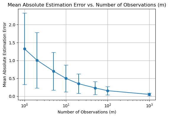
# Plotting Mean Absolute Estimation Error vs. m
plt.figure(figsize=(6, 4))
plt.errorbar(m_values, mean_abs_errors,
             yerr=std_abs_errors, fmt='o-', capsize=5)
plt.title('Mean Absolute Estimation Error vs. Number of Observations (m)')
plt.xlabel('Number of Observations (m)')
plt.ylabel('Mean Absolute Estimation Error')
plt.xscale('log')
plt.grid(True)
plt.show()

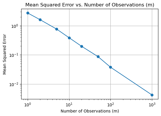
# Plotting Mean Squared Error vs. m
plt.figure(figsize=(6, 4))
plt.plot(m_values, mse_errors, 'o-', label='Mean Squared Error')
plt.title('Mean Squared Error vs. Number of Observations (m)')
plt.xlabel('Number of Observations (m)')
plt.ylabel('Mean Squared Error')
plt.xscale('log')
plt.yscale('log')
plt.grid(True)
plt.show()


# Fixed true mean
mu_true_random = np.random.normal(m1, beta)
mu_true = mu_true_random  # Fixed true mean for all simulations

# Arrays to store results
average_mu_hat_mmse = []
std_mu_hat_mmse = []

for m in m_values:
    mu_hat_mmse_values = []

    for _ in range(num_simulations):
        # Generate observed data y_k ~ N(mu_true, sigma^2)
        y = np.random.normal(mu_true, sigma, m)

        # Compute the sample mean
        y_bar = np.mean(y)

        # Compute the Bayesian MMSE estimator
        numerator = beta2 * y_bar + m1 * sigma2 / m
        denominator = beta2 + sigma2 / m
        mu_hat_mmse = numerator / denominator

        # Store the estimator
        mu_hat_mmse_values.append(mu_hat_mmse)

    # Convert list to array
    mu_hat_mmse_values = np.array(mu_hat_mmse_values)

    # Compute average and standard deviation of mu_hat_mmse
    avg_mu_hat_mmse = np.mean(mu_hat_mmse_values)
    std_mu_hat_mmse_val = np.std(mu_hat_mmse_values)

    # Store the results
    average_mu_hat_mmse.append(avg_mu_hat_mmse)
    std_mu_hat_mmse.append(std_mu_hat_mmse_val)

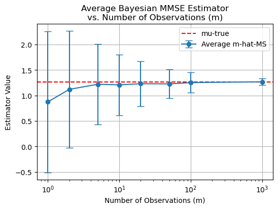
# Plotting mu_true and average mu_hat_mmse vs. m
plt.figure(figsize=(6, 4))
plt.errorbar(m_values, average_mu_hat_mmse,
             yerr=std_mu_hat_mmse, fmt='o-',
             capsize=5, label='Average m-hat-MS')
plt.axhline(mu_true, color='red', linestyle='--', label='mu-true')
plt.title('Average Bayesian MMSE Estimator\nvs. Number of Observations (m)')
plt.xlabel('Number of Observations (m)')
plt.ylabel('Estimator Value')
plt.xscale('log')
plt.legend()
plt.grid(True)
plt.show()

Discussion. Is This MMSE Estimate Biased ?#
Computing the expected value of this estimate, assuming that the parameter \(\mu\) is held constant (a realization of the unknown random parameter), results in
But the expected value of the sample mean \(\vec{y}\) for constant \(\mu\) is \(E\{\vec{y}|\mu\} = \mu\), so that
Since the expected value \(E\{\hat{\mu}_{\text{MMSE}}|\mu\}\) is not equal to \(\mu\), the estimate is biased.
However, for a large number of observations—i.e., as \(m\) becomes large—the estimate is asymptotically unbiased.
To see this, we take the expectation of \(E\{\hat{\mu}_{\text{MMSE}}|\mu\}\) again over the random variable \(\mu\), which can be stated as
where the first expectation is with respect to \(\mu\).
General Mean and Variance#
This last result is computed for a special case but is actually true in general.
To prove this result, the expected value of the estimate is obtained, i.e.,
From Eq. (C3.78) and the foregoing result, it can be seen that \(E\{\alpha_e\} = 0\) for the MSE cost function.
Therefore,
the conditional cost in Eq. (C3.80) is the conditional error variance, and
the average risk in Eq. (C3.81) is the variance of the estimation error or error variance.
The relationship can be more easily seen by writing the variance of the estimation error \(V\{\alpha_e\}\) as
This equation is actually the average risk with an MSE cost function.
Since the error variance is minimized using the MSE cost function, the estimate obtained is denoted \(\hat{\alpha}_{\text{MSE}}\) and is referred to as a minimum error-variance estimate.
Example C3.8: Average Risk \( R_{\min} \)#
The previous example can be continued by substituting the estimate into Eq. (C3.79) to obtain the average risk, \( R_{\min} \), i.e.,
Minimum Variance of the Estimation Error#
The above expression of \(R_{\min}\) is the minimum variance of the estimation error.
An alternate derivation of the preceding equation can be obtained by computing the variance of the estimation error using
where \(\mu_e = \mu - \hat{\mu}_{\text{MMSE}}\). Note that
The error variance is then
Examining the inner expectation results in
Since
it follows that
Recognizing \( V\{\vec{y}|\mu\} = \sigma^2 / m \), where \( E\{\vec{y}|\mu\} = \mu \), it can be seen that \( E\{\vec{y}^2|\mu\} = \frac{\sigma^2}{m} + \mu^2 \), so that the previous equation can be written as
and, eliminating the condition on \(\mu\), the equation becomes
Using \( E\{\mu^2\} = \beta^2 + m_1^2 \) and \( E\{\mu\} = m_1 \), the preceding equation can be reduced to
This result is the minimum variance of the estimation error expressed as \( R_{\min} \) in Example C3.8 above.
Note that the variance of the estimate \( V\{\hat{\mu}_{\text{MMSE}}\} \) can also be computed, i.e.,
Appendix#
Derivation of Equation (C3.98):
We derive the posterior probability density function (pdf) \( p(\mu | \vec{y}) \) given by:
where
\( \gamma^2 = \left( \dfrac{m}{\sigma^2} + \dfrac{1}{\beta^2} \right)^{-1} \)
\( \omega = \dfrac{m \bar{y}}{\sigma^2} + \dfrac{m_1}{\beta^2} \)
\( \bar{y} = \dfrac{1}{m} \sum_{k=1}^{m} y_k \)
Given that, the observations \( \mathbf{y}_1, \mathbf{y}_2, \ldots, \mathbf{y}_m \) are independent and normally distributed with mean \( \mu \) and known variance \( \sigma^2 \), and \(\vec{y}\) is one realization of the observation set:
The prior pdf of \( \mu \) is normal with mean \( m_1 \) and variance \( \beta^2 \):
The posterior pdf is given by:
Since \( p(\vec{y}) \) does not depend on \( \mu \), we can write:
We focus on the numerator because the denominator \( p(\vec{y}) \) serves as a normalization constant.
Combine the exponents from the likelihood and
and the prior exponent
We have the likelihood term expansion as
and the prior term expansion as
The combined exponent \( S \) is:
Combining the terms involving \( \mu^2 \), \( \mu \), and constants, we have
We can denote them collectively as \( C \), which will be absorbed into the normalization constant.
Thus, we have
To express \( S \) in the form \( -\dfrac{1}{2\gamma^2} (\mu - \mu_{\text{post}})^2 \), we complete the square.
Let
\( a = \left( \dfrac{m}{\sigma^2} + \dfrac{1}{\beta^2} \right) \)
\( b = \left( \dfrac{1}{\sigma^2} \sum_{k=1}^{m} y_k + \dfrac{m_1}{\beta^2} \right) \)
We have
and then
The term \( \frac{b^2}{2a} + C \) is a constant with respect to \( \mu \) and can be absorbed into the normalization constant.
Next, identify \( \gamma^2 \) and \( \omega \):
where
since \( \sum_{k=1}^{m} y_k = m \bar{y} \).
Substituting back into the exponent:
Therefore, the posterior pdf is:
We obtain (C3.98).
