Consistent Estimates

An estimator \( \hat{\boldsymbol{\alpha}}_m \) is said to be consistent if it converges stochastically (in probability) to the true parameter \( \alpha \) as the number of samples \( m \) becomes large.

Consistency means that as we increase the number of observations, the estimate \( \hat{\boldsymbol{\alpha}}_m \) becomes arbitrarily close to the true value \( \alpha \), with high probability.

Consistency can be expressed more rigorously through a probabilistic statement.

For any small \( \epsilon > 0 \), the probability that the estimate \( \hat{\boldsymbol{\alpha}}_m \) lies within an interval \( (\alpha - \epsilon, \alpha + \epsilon) \) around the true parameter \( \alpha \) should approach 1 as the number of observations \( m \) goes to infinity, i.e.:

\[ \boxed{ \lim_{m \to \infty} \Pr ( \alpha - \epsilon < \hat{\boldsymbol{\alpha}}_m < \alpha + \epsilon ) = 1 } \]

In other words, an estimator \( \hat{\boldsymbol{\alpha}} \) is consistent for a parameter \( \alpha \) if, as the sample size \( m \to \infty \), the probability that the estimator is within any arbitrary distance \( \epsilon \) of the true parameter approaches \(1\), i.e.:

\[ \lim_{m \to \infty} \Pr \left( |\hat{\boldsymbol{\alpha}}(\vec{y}_m) - \alpha| \leq \epsilon \right) = 1, \quad \forall \epsilon > 0 \]

Alternatively:

\[ \lim_{m \to \infty} \Pr \left(|\hat{\boldsymbol{\alpha}}(\vec{y}_m) - \alpha| \geq \epsilon \right) = 0, \quad \forall \epsilon > 0 \]

Relationship to Chebyshev’s Inequality

Consistency can also be related to Chebyshev’s inequality.

Recall that, for an unbiased estimator, Chebyshev’s inequality states that:

\[ \Pr(|\hat{\boldsymbol{\alpha}} - \alpha| > \epsilon) < \frac{V\{\hat{\boldsymbol{\alpha}}\}}{\epsilon^2} \]

where \( V\{\hat{\boldsymbol{\alpha}}\} = E\{(\hat{\boldsymbol{\alpha}} - \alpha)^2\} \) is the variance of the estimator.

If we know that the variance \( V\{\hat{\boldsymbol{\alpha}}(\vec{y}_m)\} \) converges to 0 as \( m \to \infty \), i.e.,

\[ \boxed{ \lim_{m \to \infty} V\{\hat{\boldsymbol{\alpha}}(\vec{y}_m)\} = 0 } \]

then Chebyshev’s inequality implies that \( \Pr(|\hat{\boldsymbol{\alpha}}(\vec{y}_m) - \alpha| > \epsilon) \) will also converge to 0, showing that \( \hat{\boldsymbol{\alpha}} \) is a consistent estimator.

Discussion. Dependence on Sample Size \( m \)

The subscript \( m \) is introduced to explicitly show that the estimator \( \hat{\boldsymbol{\alpha}}_m \) depends on the number of observations or random variables used to compute the estimate.

In practice, the number of observations directly affects the estimator’s accuracy, meaning that with more data, the estimator is expected to yield more accurate results.

Often, the dependence on \( m \) and on the specific sample values \( \vec{\mathbf{y}} \) is suppressed in notation for simplicity, but when discussing consistency, it’s important to recognize this dependency since increasing \( m \) is crucial for the estimator to converge to the true parameter.

Discussion. Role of \( \epsilon \)

In the formal definition of consistency, \( \epsilon \) represents any arbitrarily small positive number.

The definition requires that no matter how small \( \epsilon \) is, the probability that the estimate lies within \( \epsilon \) of the true value approaches 1 as \( m \to \infty \).

This is a very strong condition that guarantees the estimator’s reliability with a sufficiently large sample size.

Example: Sample Mean as a Consistent Estimator

To illustrate, consider the sample mean \( \bar{\mathbf{y}}_m \) as an estimator of the population mean \( \mu \). Given independent, identically distributed (i.i.d.) samples \( \mathbf{y}_1, \mathbf{y}_2, \dots, \mathbf{y}_m \), the sample mean is given by:

\[ \bar{\mathbf{y}}_m = \frac{1}{m} \sum_{i=1}^{m} \mathbf{y}_i \]

As the number of samples \( m \to \infty \), the sample mean \( \bar{\mathbf{y}}_m \) converges to the true population mean \( \mu \) by the law of large numbers.

That is, for any \( \epsilon > 0 \):

\[ \lim_{m \to \infty} \Pr(|\bar{\mathbf{y}}_m - \mu| < \epsilon) = 1 \]

\[ \lim_{m \to \infty} V\{\bar{\mathbf{y}}_m\} = 0 \]

This makes \( \bar{\mathbf{y}}_m \) a consistent estimator of \( \mu \).

Applying Chebyshev’s Inequality to the Sample Mean

We will apply Chebyshev’s Inequality to the sample mean \(\bar{\mathbf{y}}_m\) to evaluate its consistency as an estimator for the population mean \(\mu\).

The variance of the sample mean is:

\[ V\left\{ \bar{\mathbf{y}}_m \right\} = V\left\{ \frac{1}{m} \sum_{i=1}^{m} \mathbf{y}_i \right\} = \frac{1}{m^2} \sum_{i=1}^{m} V\left\{ \mathbf{y}_i \right\} = \frac{1}{m^2} \cdot m \sigma^2 = \frac{\sigma^2}{m} \]

As the sample size \(m \to \infty\), the variance of the sample mean:

\[ \lim_{m \to \infty} V\left\{ \bar{\mathbf{y}}_m \right\} = \lim_{m \to \infty} \frac{\sigma^2}{m} = 0 \]

This satisfies the condition: $\( \lim_{m \to \infty} V\{\hat{\boldsymbol{\alpha}}(\vec{y}_m)\} = 0 \)$

Thus, the sample mean is a consistent estimator for the true mean.

Moreover, we have

\[ \Pr\left( \left| \bar{\mathbf{y}}_m - \mu \right| \geq \epsilon \right) \leq \frac{V\left\{ \bar{\mathbf{y}}_m \right\}}{\epsilon^2} = \frac{\sigma^2}{m \epsilon^2} \]

Take the limit as \(m \to \infty\)

\[ \lim_{m \to \infty} \Pr\left( \left| \bar{\mathbf{y}}_m - \mu \right| \geq \epsilon \right) \leq \lim_{m \to \infty} \frac{\sigma^2}{m \epsilon^2} = 0 \]

Thus,

\[ \lim_{m \to \infty} \Pr\left( \left| \bar{\mathbf{y}}_m - \mu \right| \geq \epsilon \right) = 0 \]

equivalently,

\[ \lim_{m \to \infty} \Pr\left( \left| \bar{\mathbf{y}}_m - \mu \right| < \epsilon \right) = 1 \]

import numpy as np
import matplotlib.pyplot as plt

# Set random seed for reproducibility
np.random.seed(42)

# 1. Assumptions
mu = 10.0             # True population mean
sigma2 = 4.0         # Known variance of observations (σ²)
sigma = np.sqrt(sigma2)  # Standard deviation
epsilon = 1.0        # Epsilon for probability calculation

# 2. Simulation Parameters
sample_sizes = [10, 20, 30, 40, 50, 100, 200]  # Different sample sizes to test
num_trials = 10000      # Number of trials for each sample size

# Initialize lists to store results
probabilities = []            # Pr(|\mathbf{y}_bar - mu| < epsilon)
empirical_variances = []      # Empirical variance of \mathbf{y}_bar
chebyshev_bounds = []         # Chebyshev's bound for each m

# 3. Simulation Loop
for m in sample_sizes:
    # 2. Generate m samples for each trial: shape (num_trials, m)
    samples = np.random.normal(loc=mu, scale=sigma, size=(num_trials, m))
    
    # 3. Compute the sample mean for each trial: shape (num_trials,)
    sample_means = np.mean(samples, axis=1)
    
    # 4. Compute the probability Pr(|\mathbf{y}_bar - mu| < epsilon)
    # This is the proportion of sample_means within [mu - epsilon, mu + epsilon]
    count_within_epsilon = np.sum(np.abs(sample_means - mu) < epsilon)
    probability = count_within_epsilon / num_trials
    probabilities.append(probability)
    
    # 5. Compute the empirical variance of the sample means
    empirical_var = np.var(sample_means, ddof=1)
    empirical_variances.append(empirical_var)
    
    # Compute Chebyshev's bound: sigma² / (m * epsilon²)
    chebyshev_bound = sigma2 / (m * epsilon**2)
    chebyshev_bounds.append(chebyshev_bound)
    
    # Optional: Print progress
    # print(f"Sample Size m = {m}:")
    # print(f"  Pr(|\mathbf{y}_bar - mu| < {epsilon}) = {probability:.4f}")
    # print(f"  Empirical Variance of \mathbf{y}_bar = {empirical_var:.4f}")
    # print(f"  Chebyshev's Bound = {chebyshev_bound:.4f}\n")

# 4. Visualization

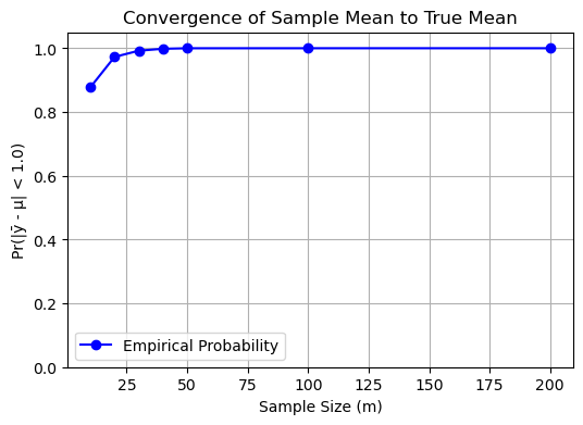
# a. Probability Pr(|\mathbf{y}_bar - mu| < epsilon) vs. Sample Size m
plt.figure(figsize=(6, 4))
plt.plot(sample_sizes, probabilities, marker='o', linestyle='-', color='blue', label='Empirical Probability')
plt.xlabel('Sample Size (m)')
plt.ylabel(f'Pr(|ȳ - μ| < {epsilon})')
plt.title('Convergence of Sample Mean to True Mean')
plt.ylim(0, 1.05)
plt.grid(True)
plt.legend()
plt.show()

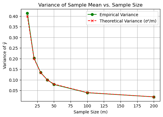
# b. Empirical Variance of \mathbf{y}_bar vs. Sample Size m
plt.figure(figsize=(6, 4))
plt.plot(sample_sizes, empirical_variances, marker='o', linestyle='-', color='green', label='Empirical Variance')
plt.plot(sample_sizes, [sigma2/m for m in sample_sizes], marker='x', linestyle='--', color='red', label='Theoretical Variance (σ²/m)')
plt.xlabel('Sample Size (m)')
plt.ylabel('Variance of ȳ')
plt.title('Variance of Sample Mean vs. Sample Size')
plt.grid(True)
plt.legend()
plt.show()

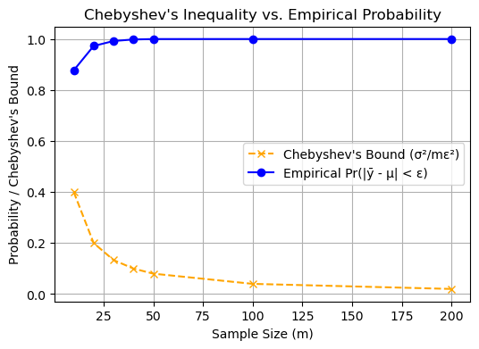
# c. Chebyshev's Bound vs. Empirical Probability
plt.figure(figsize=(6, 4))
plt.plot(sample_sizes, chebyshev_bounds, marker='x', linestyle='--', color='orange', label="Chebyshev's Bound (σ²/mε²)")
plt.plot(sample_sizes, probabilities, marker='o', linestyle='-', color='blue', label='Empirical Pr(|ȳ - μ| < ε)')
plt.xlabel('Sample Size (m)')
plt.ylabel('Probability / Chebyshev\'s Bound')
plt.title('Chebyshev\'s Inequality vs. Empirical Probability')
plt.grid(True)
plt.legend()
plt.show()

Invariant Estimators

An important characteristic that an estimator is invariance under transformations of the parameter being estimated.

Formally, consider an estimator \( \hat{\boldsymbol{\alpha}} \) of a parameter \( \alpha \), and let \( g(\alpha) \) be a function of \( \alpha \).

The estimator \( \hat{\boldsymbol{\alpha}} \) is said to be invariant under the transformation \( g \) if \( g(\hat{\boldsymbol{\alpha}}) \) serves as a (good) estimator of \( g(\alpha) \).

This typically means that \( g(\hat{\boldsymbol{\alpha}}) \) retains desirable properties such as unbiasedness or consistency when estimating \( g(\alpha) \).

For instance, maximum likelihood estimators (MLEs) exhibit this invariance property.

Specifically, if \( \hat{\boldsymbol{\alpha}}_{\text{MLE}} \) is the MLE of \( \alpha \), then \( g(\hat{\boldsymbol{\alpha}}_{\text{MLE}}) \) is the MLE of \( g(\alpha) \).

Example: Sample Mean Squared Estimator

Consider independent and identically distributed (i.i.d.) random variables \( \mathbf{y}_1, \mathbf{y}_2, \dots, \mathbf{y}_m \), each with mean \( \mu \) and variance 1; that is, \( E[\mathbf{y}_i] = \mu \) and \( \operatorname{Var}(\mathbf{y}_i) = 1 \) for all \( i \).

The sample mean is defined as:

\[ \hat{\boldsymbol{\mu}} = \frac{1}{m} \sum_{i=1}^m \mathbf{y}_i \]

This estimator is unbiased since:

\[ E[\hat{\boldsymbol{\mu}}] = \frac{1}{m} \sum_{i=1}^m E[\mathbf{y}_i] = \frac{1}{m} \cdot m \mu = \mu \]

Now, consider the function \( g(\mu) = \mu^2 \) and its estimator \( g(\hat{\boldsymbol{\mu}}) = \hat{\boldsymbol{\mu}}^2 \).

One might expect \( \hat{\boldsymbol{\mu}}^2 \) to be a good estimator of \( \mu^2 \), but let’s examine its properties.

Compute the expected value of \( \hat{\boldsymbol{\mu}}^2 \):

\[ E[\hat{\boldsymbol{\mu}}^2] = E\left[ \left( \frac{1}{m} \sum_{i=1}^m \mathbf{y}_i \right)^2 \right] = \operatorname{Var}(\hat{\boldsymbol{\mu}}) + \left( E[\hat{\boldsymbol{\mu}}] \right)^2 \]

Since \( \operatorname{Var}(\hat{\boldsymbol{\mu}}) = \frac{1}{m^2} \sum_{i=1}^m \operatorname{Var}(\mathbf{y}_i) = \frac{1}{m^2} \cdot m \cdot 1 = \frac{1}{m} \), we have:

\[ E[\hat{\boldsymbol{\mu}}^2] = \frac{1}{m} + \mu^2 \]

This shows that \( \hat{\boldsymbol{\mu}}^2 \) is a biased estimator of \( \mu^2 \) because:

\[ E[\hat{\boldsymbol{\mu}}^2] \neq \mu^2 \]

Therefore, the invariance property does not hold in this case, as \( g(\hat{\boldsymbol{\mu}}) \) is not an unbiased estimator of \( g(\mu) \).

Example: Linear Transformation of Estimator

Now, consider a linear transformation, such as converting measurements from pounds to kilograms or seconds to minutes. Let’s revisit the sample mean \( \hat{\boldsymbol{\mu}} \) of the random variables \( \mathbf{y}_i \).

Suppose we multiply each observation by a scalar \( a \), defining new variables \( z_i = a \mathbf{y}_i \). The sample mean of the transformed data is:

\[ \hat{\boldsymbol{\mu}}_z = \frac{1}{m} \sum_{i=1}^m z_i = \frac{1}{m} \sum_{i=1}^m a \mathbf{y}_i = a \hat{\boldsymbol{\mu}} \]

The expected value of \( \hat{\boldsymbol{\mu}}_z \) is:

\[ E[\hat{\boldsymbol{\mu}}_z] = a E[\hat{\boldsymbol{\mu}}] = a \mu \]

which means \( \hat{\boldsymbol{\mu}}_z \) is an unbiased estimator of \( a \mu \).

In this case, the estimator is invariant under the transformation \( g(\mu) = a \mu \) because applying the transformation to the estimator yields an unbiased estimator of the transformed parameter:

\[ g(\hat{\boldsymbol{\mu}}) = a \hat{\boldsymbol{\mu}} \quad \text{is an unbiased estimator of} \quad g(\mu) = a \mu \]

Thus, invariance is achieved under linear scaling transformations.