MAP and ML Criteria

Hypothesis Testing

Consider two possible values \( s_0 \) and \( s_1 \).

We aim to decide between these two alternatives when we observe a measurement \( \mathbf{y} \) corrupted by noise \( \mathbf{n} \).

That is, we observe

\[ \mathbf{y} = s_i + \mathbf{n}, \quad i = 0, 1 \]

and decide which \( s_i \) is the most likely value.

Most of the development of this section presumes a continuous measurement \( y \). This is merely a convenience, because \( y \) can just as easily represent discrete measurements. The theory is entirely consistent.

In this binary case, there are two alternative hypotheses.

• Hypothesis \( H_0 \) corresponds to \( s_0 \) is transmitted

• Hypothesis \( H_1 \) corresponds to \( s_1 \) is transmitted

MAP Criterion

We aim to determine \( P(H_i | y) \), \( i = 0, 1 \), which represents the posterior probability of each hypothesis given the observation \( y \).

Specifically, if

\[ P(H_0 | y) > P(H_1 | y) \]

we decide that hypothesis \( H_0 \) (corresponding to signal \( s_0 \)) is true.

Conversely, if

\[ P(H_1 | y) > P(H_0 | y) \]

we decide that hypothesis \( H_1 \) (corresponding to signal \( s_1 \)) is true.

Using Bayes’ theorem, the posterior probabilities can be expressed as:

\[ P(H_0 | y) = \frac{p(y | H_0) P(H_0)}{p(y)} \]

where \( P(H_i) \) is the prior probability of hypothesis \( H_i \), and \( p(y) \) is the total probability of observation \( y \). By the law of total probability, \( p(y) \) can be written as

\[ p(y) = p(y | H_0) P(H_0) + p(y | H_1) P(H_1) \]

Similarly, the posterior for \( H_1 \) is:

\[ P(H_1 | y) = \frac{p(y | H_1) P(H_1)}{p(y)} \]

The likelihood functions \( p(y | H_0) \) and \( p(y | H_1) \) represent the probability density of \( y \) given each hypothesis. Specifically,

\[ p(y | H_0) = p_{\mathbf{n}}(y - s_0) \]

and

\[ p(y | H_1) = p_{\mathbf{n}}(y - s_1) \]

where \( p_{\mathbf{n}}(\cdot) \) denotes the probability density function of the noise.

Thus, to compute the posterior probabilities \( P(H_i | y) \), \( i = 0, 1 \), we need to know the prior probabilities \( P(H_0) \) and \( P(H_1) \).

Let \( P(H_0) = \pi_0 \) and \( P(H_1) = \pi_1 \). Based on these prior probabilities, we decide that hypothesis \( H_0 \) is correct if

\[ p(y | H_0) \pi_0 > p(y | H_1) \pi_1 \]

Otherwise, we decide that hypothesis \( H_1 \) is correct.

Define:

• \( D_0 \) as the decision to select \( H_0 \),

• \( D_1 \) as the decision to select \( H_1 \).

Throughout this chapter, we will express the decision rule for choosing between \( D_0 \) and \( D_1 \) as:

\[\begin{split} \frac{p(y | H_1)}{p(y | H_0)} \begin{array}{c} D_1 \\ \gtrless \\ D_0 \end{array} \frac{\pi_0}{\pi_1} \end{split}\]

Likelihood Ratio

The likelihood ratio, which simplifies the decision-making process, is defined as:

\[ L(y) = \frac{p(y | H_1)}{p(y | H_0)} \]

MAP Threshold

The MAP threshold is defined as:

\[ \tau_{MAP} \triangleq \frac{\pi_0}{\pi_1} \]

For a given detection experiment, the ratio \( \frac{\pi_0}{\pi_1} \) represents a fixed value determined by the prior probabilities \( \pi_0 \) and \( \pi_1 \).

Consequently, the threshold \( \tau_{MAP} \) is also fixed and is specifically associated with this MAP detection experiment.

MAP Decision Procedure

1. Compute the threshold \( \tau_{MAP} \) based on the given prior probabilities \( \pi_0 \) and \( \pi_1 \): $\( \tau_{MAP} = \frac{\pi_0}{\pi_1} \)$

2. Compute the likelihood ratio expression \( L(y) = \frac{p(y|H_1)}{p(y|H_0)} \), either

• directly from the distribution of \( \mathbf{y} \), or

• indirectly from the distribution of the noise \( \mathbf{n} \) (if \( \mathbf{y} \) is a function of the noise and the signal). This step involves using the known probability density functions for \( p(y|H_0) \) and \( p(y|H_1) \) based on the system model.

3. For a specific value of the observation \( y \):

• Compare \( L(y) \) with \( \tau_{MAP} \).

• If it’s easier to work directly with \( y \), we can transform the comparison into an equivalent one between \( y \) and some function of \( \tau_{MAP} \), i.e., solve \( L(y) = \tau_{MAP} \) for \( y \), yielding a decision threshold \( y_{th} \) such that:

  \[\begin{split} y \begin{array}{c} H_1 \\ \gtrless \\ H_0 \end{array} y_{th} \end{split}\]

  Here, \( y_{th} = \mathrm{func}^{-1}(\tau_{MAP}) \), where \( \mathrm{func}^{-1}(\cdot) \) represents the inverse of the likelihood ratio function.

This final step allows us to directly compare the observation \( y \) with the transformed threshold \( y_{th} \), simplifying the decision process.

Discussion.

• To obtain \( \mathrm{func}^{-1} \), the likelihood ratio function \( L(y) = \frac{p(y|H_1)}{p(y|H_0)} \) needs to be invertible, but differentiability is not strictly required. The key requirement is that the likelihood ratio function should be monotonic over the range of interest so that it can be inverted.

• In cases where \( L(y) = \tau_{MAP} \), the MAP criterion does not specify which hypothesis to choose. Other detection criteria, discussed later in the chapter, address this ambiguity.

• When \( L(y) = \tau_{MAP} \), no decision is made. However, by convention, we will choose hypothesis \( H_1 \) when \( L(y) \geq \tau_{MAP} \).

Maximum-Likelihood Criterion

In detection theory, when the two hypotheses (\( H_0 \) and \( H_1 \)) are equally likely a priori, it means that the prior probabilities are the same, i.e.,

\[ \pi_0 = \pi_1 \]

recall that \( \pi_0 \) and \( \pi_1 \) represent the prior probabilities of hypotheses \( H_0 \) and \( H_1 \), respectively.

Under this condition, the decision threshold for the maximum a posteriori (MAP) criterion, denoted as \( \tau_{MAP} \), simplifies to:

\[ \tau_{MAP} = 1 \]

This leads to a special case known as the maximum-likelihood (ML) criterion, where the threshold for deciding between the two hypotheses is:

\[ \tau_{ML} = 1 \]

The ML criterion is frequently used when there is no information available about the a priori probabilities. However, in such cases, analysts are often advised to consider the minimax criterion, which minimizes the maximum risk across different decisions.

Despite this, the ML criterion remains highly valuable in estimation theory, as it is effective when the goal is to estimate parameters based on observed data without relying on prior knowledge.

Exmaple: Antipodal Signal Detection and Decision Process

Problem Statement

In this example [B2, Ex 4.1], we consider antipodal signals where \( s_0 = -b \) and \( s_1 = b \), with the a priori probabilities \( \pi_0 = 0.8 \) and \( \pi_1 = 0.2 \), respectively. We assume \( b > 0 \).

The noise \( \mathbf{n} \) is modeled as a zero-mean Gaussian random variable with variance \( \sigma^2 \).

The probability density function (pdf) of the noise is:

\[ p_{\mathbf{n}}(n) = \frac{1}{\sqrt{2\pi\sigma^2}} \exp\left( -\frac{n^2}{2\sigma^2} \right) \]

Likelihood Functions

Given the observation \( y \), the likelihood functions under the two hypotheses are:

\[ p(y|H_1) = \frac{1}{\sqrt{2\pi\sigma^2}} \exp\left( -\frac{(y - b)^2}{2\sigma^2} \right) \]

\[ p(y|H_0) = \frac{1}{\sqrt{2\pi\sigma^2}} \exp\left( -\frac{(y + b)^2}{2\sigma^2} \right) \]

Detection using MAP Criterion

To apply the Maximum A Posteriori (MAP) criterion, we need to compare the likelihood ratio \( L(y) \) to the threshold \( \tau_{MAP} \):

\[ \tau_{MAP} = \frac{\pi_0}{\pi_1} = \frac{0.8}{0.2} = 4 \]

The likelihood ratio is:

\[ L(y) = \frac{p(y|H_1)}{p(y|H_0)} = \exp\left[ \frac{(y + b)^2 - (y - b)^2}{2\sigma^2} \right] = \exp\left( \frac{2yb}{\sigma^2} \right) \]

Decision Rule

We decide \( H_1 \) if:

\[ L(y) \geq \tau_{MAP} \iff \exp\left( \frac{2yb}{\sigma^2} \right) \geq 4 \]

Taking the natural logarithm of both sides, we get:

\[ \frac{2yb}{\sigma^2} \geq \ln 4 \]

\[ y \geq \frac{\sigma^2 \ln 4}{2b} \]

Numerical Example

For example, if \( b = 1 \) and \( \sigma^2 = 0.25 \), the decision rule becomes:

\[ y \geq \frac{0.25 \ln 4}{2 \cdot 1} = 0.173287 \]

Discussion.

Here’s the corrected version of your statement:

If the a priori probabilities are equal (\( \pi_0 = \pi_1 = 0.5 \)), then the MAP threshold \( \tau_{MAP} \) becomes 1. In this case, we decide \( H_1 \) if:

\[ L(y) \geq \tau_{MAP} \iff \exp\left( \frac{2yb}{\sigma^2} \right) \geq 1 \]

This simplifies to a decision rule based purely on the likelihood ratio, i.e., \( y \geq 0 \), since \( \ln 1 = 0 \).

This is why the ML (Maximum Likelihood) criterion is effective when we do not have prior knowledge of the probabilities, as it relies solely on the likelihood of the observation without incorporating prior probabilities.

Numerical Results

import numpy as np

# Given parameters
b = 1
sigma = 0.5 # std, thus, variance sigma^2 = 0.25
pi0 = 0.8
pi1 = 0.2

# Number of simulations, should be 1e6 to get accurate results
n_samples = 1000000

# Generating s0 and s1
s0 = -b
s1 = b

# Generating noise
noise = np.random.normal(0, np.sqrt(sigma**2), n_samples)

# Simulating received y under each hypothesis
y_given_s0 = s0 + noise
y_given_s1 = s1 + noise

# MAP criterion threshold
tau_MAP = np.log(pi0 / pi1)

# Decision rule based on MAP criterion
# Likelihood ratio test: exp(2yb / sigma**2) >= pi0 / pi1
# Taking log: 2yb / sigma**2 >= log(pi0 / pi1)
# Decision threshold: y >= (sigma**2 / (2b)) * log(pi0 / pi1)
threshold = (sigma**2 / (2 * b)) * tau_MAP

# Decisions
decisions_s0 = y_given_s0 >= threshold
decisions_s1 = y_given_s1 >= threshold

# Estimating transmitted signals (s_hat) based on decisions
s0_hat = np.where(decisions_s0, s1, s0)  # Decided s1 if decision is True, else s0
s1_hat = np.where(decisions_s1, s1, s0)

# Compute MSE for both cases
mse_s0 = np.mean((s0_hat - s0) ** 2)
mse_s1 = np.mean((s1_hat - s1) ** 2)

mse_s0, mse_s1

(np.float64(0.038468), np.float64(0.197924))

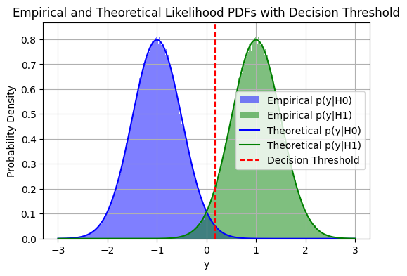
Plot theoretical and empirical PDFs

# Re-importing necessary libraries
import numpy as np
import matplotlib.pyplot as plt

# Empirical PDFs
bins = np.linspace(-3, 3, 1000)  # Adjust this range based on your data range
empirical_pdf_H0, _ = np.histogram(y_given_s0, bins=bins, density=True)  # Histogram for H0
empirical_pdf_H1, _ = np.histogram(y_given_s1, bins=bins, density=True)  # Histogram for H1
y_values_mid = (bins[:-1] + bins[1:]) / 2  # Midpoints of bins for plotting

# Manual calculation of Theoretical PDFs
def gaussian_pdf(y, mu, sigma):
    """Calculate the Gaussian PDF."""
    return (1 / np.sqrt(2 * np.pi * sigma**2)) * np.exp(-((y - mu)**2) / (2 * sigma**2))

# Theoretical PDFs for H0 and H1 using the manual Gaussian formula
theoretical_pdf_H0 = gaussian_pdf(y_values_mid, mu=s0, sigma=sigma)  # for H0 hypothesis
theoretical_pdf_H1 = gaussian_pdf(y_values_mid, mu=s1, sigma=sigma)  # for H1 hypothesis

# Plotting
plt.figure(figsize=(6, 4))

# Plotting Empirical PDFs as histograms
plt.hist(y_given_s0, bins=bins, density=True, alpha=0.5, label='Empirical p(y|H0)', color='blue')
plt.hist(y_given_s1, bins=bins, density=True, alpha=0.5, label='Empirical p(y|H1)', color='green')

# Theoretical PDFs with solid lines (manually computed using the Gaussian formula)
plt.plot(y_values_mid, theoretical_pdf_H0, label='Theoretical p(y|H0)', linestyle='solid', color='blue')
plt.plot(y_values_mid, theoretical_pdf_H1, label='Theoretical p(y|H1)', linestyle='solid', color='green')

# Decision threshold line
plt.axvline(x=threshold, color='red', linestyle='--', label='Decision Threshold')

# Labels and legend
plt.xlabel('y')
plt.ylabel('Probability Density')
plt.title('Empirical and Theoretical Likelihood PDFs with Decision Threshold')
plt.legend()
plt.grid(True)
plt.show()

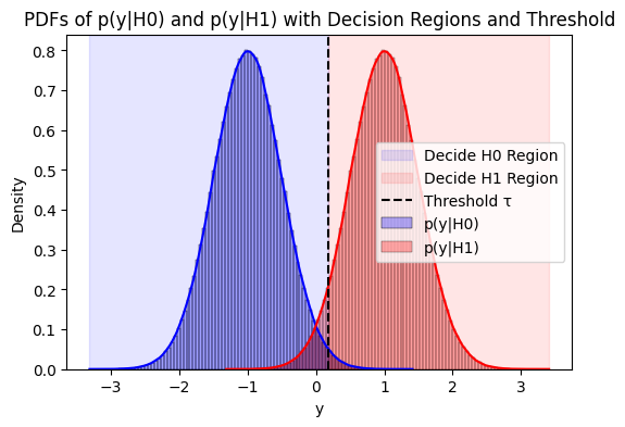
Plot decision regions

import seaborn as sns

# Plot PDFs and shading decision regions
plt.figure(figsize=(6, 4))

# PDF under H0 (p(y|H0))
sns.histplot(y_given_s0, bins=100, kde=True, stat="density", label="p(y|H0)", color="blue", alpha=0.3)

# PDF under H1 (p(y|H1))
sns.histplot(y_given_s1, bins=100, kde=True, stat="density", label="p(y|H1)", color="red", alpha=0.3)

# Shading the decision regions
plt.axvspan(xmin=min(y_given_s0), xmax=threshold, color='blue', alpha=0.1, label='Decide H0 Region')
plt.axvspan(xmin=threshold, xmax=max(y_given_s1), color='red', alpha=0.1, label='Decide H1 Region')

# Plot the decision threshold
plt.axvline(x=threshold, color='black', linestyle='--', label='Threshold τ')

# Labels and title
plt.xlabel('y')
plt.ylabel('Density')
plt.title('PDFs of p(y|H0) and p(y|H1) with Decision Regions and Threshold')
plt.legend()

# Show the plot
plt.show()

Decision Rule

By definition,

• \( D_0 \) is associated with the range of the observation \( y \) such that \( L(y) < \tau_{MAP} \).

• \( D_1 \) is associated with the range of \( y \) for which \( L(y) \geq \tau_{MAP} \).

Let \( R_0 \) and \( R_1 \) be each of these ranges of \( y \), respectively.

A decision rule \( \delta(y) \) can be defined as

\[\begin{split} \delta(y) = \begin{cases} 1, & y \in R_1 \\ 0, & y \in R_0 \end{cases} \end{split}\]

In terms of the MAP criterion, \( y \) is in \( R_1 \) if

\[ y \in R_1 \implies L(y) \geq \frac{\pi_0}{\pi_1} \]

and

\[ y \in R_0 \implies L(y) < \frac{\pi_0}{\pi_1} \]

It follows that the MAP decision rule is

\[\begin{split} \delta_{MAP}(y) = \begin{cases} 1, & \forall y \ni L(y) \geq \frac{\pi_0}{\pi_1} \\ 0, & \forall y \ni L(y) < \frac{\pi_0}{\pi_1} \end{cases} \end{split}\]

Types of Errors

Consider the case where, under hypothesis \( H_0 \), \( s_0 = 0 \). This situation is closely related to the classical radar case. A radar illuminates a specific volume of space.

The return signal can be modeled in terms of two hypotheses:

• \( H_0 \) corresponds to “no signal”

• \( H_1 \) corresponds to “signal present.”

In this case, \( H_0 \) is often referred to as the null hypothesis and \( H_1 \) as the alternate hypothesis.

We define \( P_{ij} \) as the probability of deciding \( D_i \), when, in fact, hypothesis \( H_j \) is correct.

In terms of the underlying probability density functions, it can be seen that

\[ P_{ij} = \int_{R_i} p(y|H_j) \, dy \]

where the integral is understood to include the cases where the density functions are discrete or hybrid.

For binary hypotheses, some historical radar terminology is often used for three of these probabilities.

• \( P_{01} \) is often called the probability of a “miss,” \( P_m \). That is, a signal is present (\( H_1 \) is correct) and we have missed it by deciding \( D_0 \).

• \( P_{11} \) is called the probability of detection \( P_d \). That is, we decide a signal is present and it actually is.

• \( P_{10} \), the probability of deciding \( D_1 \) (a signal is present) when \( H_0 \) is correct (no signal present), is called the probability of a “false alarm,” \( P_f \).

• \( P_{00} \) was too mundane for radar technologists to give it a special name.

Only two of these probabilities correspond to errors, namely \( P_{01} \) and \( P_{10} \).

In many applications (communications, for example), we are more interested in the average error probability

\[ P_E = \pi_0 P_{10} + \pi_1 P_{01} \]

Example: Types of Errors when using MAP decision rule with log-likelihood threshold

This example [B2, Ex 4.3] is an extension of the previous example, i.e., antipodal signal detection example.

We define some additional terminology and observe the various decision regions for this example.

If we define a log-likelihood threshold as \( \tau' \), then the four terms \( P_{ij}, i = 0, 1, j = 0, 1 \), can be written as

\[ P_{00} = \int_{-\infty}^{\tau'} \frac{1}{\sqrt{2\pi\sigma^2}} \exp\left(-\frac{(y + b)^2}{2\sigma^2}\right) dy \]

\[ P_{01} = \int_{-\infty}^{\tau'} \frac{1}{\sqrt{2\pi\sigma^2}} \exp\left(-\frac{(y - b)^2}{2\sigma^2}\right) dy \]

\[ P_{10} = \int_{\tau'}^{\infty} \frac{1}{\sqrt{2\pi\sigma^2}} \exp\left(-\frac{(y + b)^2}{2\sigma^2}\right) dy \]

\[ P_{11} = \int_{\tau'}^{\infty} \frac{1}{\sqrt{2\pi\sigma^2}} \exp\left(-\frac{(y - b)^2}{2\sigma^2}\right) dy \]

Error function and complementary error function

\[ \text{erf}(z) = \frac{2}{\sqrt{\pi}} \int_{0}^{z} e^{-t^2} dt \]

and

\[ \text{erfc}(z) = \frac{2}{\sqrt{\pi}} \int_{z}^{\infty} e^{-t^2} dt = 1 - \text{erf}(z) \]

and making the appropriate changes of variables, we can write

\[ P_{00} = \frac{1}{2} \left[ 1 + \text{erf} \left( \frac{\tau' + b}{\sqrt{2\sigma^2}} \right) \right] \]

\[ P_{01} = \frac{1}{2} \left[ 1 + \text{erf} \left( \frac{\tau' - b}{\sqrt{2\sigma^2}} \right) \right] \]

\[ P_{10} = \frac{1}{2} \text{erfc} \left( \frac{\tau' + b}{\sqrt{2\sigma^2}} \right) \]

\[ P_{11} = \frac{1}{2} \text{erfc} \left( \frac{\tau' - b}{\sqrt{2\sigma^2}} \right) \]

We can see that the MAP decision rule is

\[\begin{split} \delta_{MAP}(y) = \begin{cases} 1, & y \geq \frac{\sigma^2}{2b} \ln 4 \\ 0, & y < \frac{\sigma^2}{2b} \ln 4 \end{cases} \end{split}\]

where the decision regions are

\[ R_1 = \{ y : y \geq \frac{\sigma^2}{2b} \ln 4 \} \]

\[ R_0 = \{ y : y < \frac{\sigma^2}{2b} \ln 4 \} \]

It follows that for the MAP criterion,

\[ \tau' = \frac{\sigma^2}{2b} \ln \tau_{MAP} = \frac{\sigma^2}{2b} \ln \frac{\pi_0}{\pi_1} = \frac{\sigma^2}{2b} \ln 4 \]

In case of the specific settings with \( b = 1 \) and \( \sigma^2 = 0.25 \), we have

\[ P_{00} \approx 0.990526 \]

\[ P_{01} \approx 0.049122 \]

\[ P_{10} \approx 0.009474 \]

\[ P_{11} \approx 0.950878 \]

# Calculating empirical probabilities
P00_empirical_MAP = np.mean(s0_hat_MAP == s0)  # Probability of deciding H0 when H0 is true
P01_empirical_MAP = np.mean(s1_hat_MAP == s0)  # Probability of deciding H0 when H1 is true
P10_empirical_MAP = np.mean(s0_hat_MAP == s1)  # Probability of deciding H1 when H0 is true
P11_empirical_MAP = np.mean(s1_hat_MAP == s1)  # Probability of deciding H1 when H1 is true

# Print results
print(f"MAP, P00 (Decide H0 | H0 true): {P00_empirical_MAP:.4f}")
print(f"MAP, P01 (Decide H0 | H1 true): {P01_empirical_MAP:.4f}")
print(f"MAP, P10 (Decide H1 | H0 true): {P10_empirical_MAP:.4f}")
print(f"MAP, P11 (Decide H1 | H1 true): {P11_empirical_MAP:.4f}")

MAP, P00 (Decide H0 | H0 true): 0.9898
MAP, P01 (Decide H0 | H1 true): 0.0489
MAP, P10 (Decide H1 | H0 true): 0.0102
MAP, P11 (Decide H1 | H1 true): 0.9511

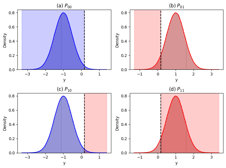
The following plots illustrate the Probability Density Functions (PDFs) for \( p(y|H_0) \) and \( p(y|H_1) \), along with the decision regions and threshold \( \tau \):

• (a) \( P_{00} \): The shaded blue region under \( p(y|H_0) \) indicates the probability of deciding \( H_0 \) when \( H_0 \) is true.

• (b) \( P_{01} \): The shaded red region under \( p(y|H_1) \) indicates the probability of deciding \( H_0 \) when \( H_1 \) is true.

• (c) \( P_{10} \): The shaded red region under \( p(y|H_0) \) indicates the probability of deciding \( H_1 \) when \( H_0 \) is true.

• (d) \( P_{11} \): The shaded red region under \( p(y|H_1) \) indicates the probability of deciding \( H_1 \) when \( H_1 \) is true.

The vertical dashed black line represents the decision threshold \( \tau \), separating the decision regions for \( H_0 \) and \( H_1 \).

# Plot PDFs and decision regions
plt.figure(figsize=(8, 6))

# P00 plot
plt.subplot(2, 2, 1)
sns.histplot(y_given_s0, bins=100, kde=True, stat="density", color="blue", alpha=0.3)
plt.axvline(x=threshold, color='black', linestyle='--')
plt.axvspan(xmin=min(y_given_s0), xmax=threshold, color='blue', alpha=0.2)
plt.xlabel('y')
plt.title('(a) $P_{00}$')

# P01 plot
plt.subplot(2, 2, 2)
sns.histplot(y_given_s1, bins=100, kde=True, stat="density", color="red", alpha=0.3)
plt.axvline(x=threshold, color='black', linestyle='--')
plt.axvspan(xmin=min(y_given_s1), xmax=threshold, color='red', alpha=0.2)
plt.xlabel('y')
plt.title('(b) $P_{01}$')

# P10 plot
plt.subplot(2, 2, 3)
sns.histplot(y_given_s0, bins=100, kde=True, stat="density", color="blue", alpha=0.3)
plt.axvline(x=threshold, color='black', linestyle='--')
plt.axvspan(xmin=threshold, xmax=max(y_given_s0), color='red', alpha=0.2)
plt.xlabel('y')
plt.title('(c) $P_{10}$')

# P11 plot
plt.subplot(2, 2, 4)
sns.histplot(y_given_s1, bins=100, kde=True, stat="density", color="red", alpha=0.3)
plt.axvline(x=threshold, color='black', linestyle='--')
plt.axvspan(xmin=threshold, xmax=max(y_given_s1), color='red', alpha=0.2)
plt.xlabel('y')
plt.title('(d) $P_{11}$')

# Adjust layout and show plot
plt.tight_layout()
plt.show()

Error Types for a general decision threshold

The threshold \(\tau\) can represent any decision threshold, not necessarily the one specific to the MAP criterion. Here are the revised expressions with \(\tau\) as the general threshold:

\( P_{00} \): Probability of deciding \( H_0 \) when \( H_0 \) is true

\[ P_{00} = \Pr(\text{Deciding } H_0 \mid H_0 \text{ is true}) = \int_{-\infty}^{\tau} p(y|H_0) \, dy \]

\( P_{01} \): Probability of deciding \( H_0 \) when \( H_1 \) is true

\[ P_{01} = \Pr(\text{Deciding } H_0 \mid H_1 \text{ is true}) = \int_{-\infty}^{\tau} p(y|H_1) \, dy \]

\( P_{10} \): Probability of deciding \( H_1 \) when \( H_0 \) is true

\[ P_{10} = \Pr(\text{Deciding } H_1 \mid H_0 \text{ is true}) = \int_{\tau}^{\infty} p(y|H_0) \, dy \]

\( P_{11} \): Probability of deciding \( H_1 \) when \( H_1 \) is true

\[ P_{11} = \Pr(\text{Deciding } H_1 \mid H_1 \text{ is true}) = \int_{\tau}^{\infty} p(y|H_1) \, dy \]

In these expressions, \(\tau\) represents the decision threshold that determines the decision rule for deciding between \( H_0 \) and \( H_1 \). This threshold can vary depending on the criteria used (such as MAP, ML, Neyman-Pearson, etc.).

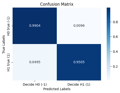
Confusion matrix

The confusion matrix provides a summary of prediction results, and these elements can be used to compute various performance metrics, such as accuracy, precision, recall, and F1 score.

In the context of decision-making, particularly in binary classification, the terms \( P_{00} \), \( P_{01} \), \( P_{10} \), and \( P_{11} \) correspond to components in a confusion matrix. The confusion matrix consists of True Positives (TP), True Negatives (TN), False Positives (FP), and False Negatives (FN). Here’s how they correspond:

• \( P_{00} \): Probability of deciding \( H_0 \) when \( H_0 \) is true.

  • Equivalent to True Negatives (TN): Correctly identifying the negative class.

• \( P_{01} \): Probability of deciding \( H_0 \) when \( H_1 \) is true.

  • Equivalent to False Negatives (FN): Incorrectly identifying the positive class as negative.

• \( P_{10} \): Probability of deciding \( H_1 \) when \( H_0 \) is true.

  • Equivalent to False Positives (FP): Incorrectly identifying the negative class as positive.

• \( P_{11} \): Probability of deciding \( H_1 \) when \( H_1 \) is true.

  • Equivalent to True Positives (TP): Correctly identifying the positive class.

# Create the confusion matrix
confusion_matrix = np.array([
    [P00_empirical, P01_empirical],
    [P10_empirical, P11_empirical]
])

# Round the values to four decimal places
confusion_matrix = np.round(confusion_matrix, 4)

# Display the confusion matrix
print("Confusion Matrix:")
print("[[P00 (Decide H0 | H0 true)  P01 (Decide H0 | H1 true)]")
print(" [P10 (Decide H1 | H0 true)  P11 (Decide H1 | H1 true)]]")
print(confusion_matrix)

Confusion Matrix:
[[P00 (Decide H0 | H0 true)  P01 (Decide H0 | H1 true)]
 [P10 (Decide H1 | H0 true)  P11 (Decide H1 | H1 true)]]
[[0.9905 0.0095]
 [0.0516 0.9484]]

from sklearn.metrics import confusion_matrix

# Combine the original transmitted signals and the estimated signals
original_signals = np.concatenate((np.full(n_samples, s0), np.full(n_samples, s1)))
decided_signals = np.concatenate((s0_hat, s1_hat))

# Create the confusion matrix
cm = confusion_matrix(original_signals, decided_signals, labels=[s0, s1])

# Normalize the confusion matrix to get probabilities
cm_normalized = cm.astype('float') / cm.sum(axis=1)[:, np.newaxis]

# Round the values to four decimal places
cm_normalized = np.round(cm_normalized, 4)

# Print the confusion matrix
print("Confusion Matrix (using sklearn):")
print("[[P00 (Decide H0 | H0 true)  P01 (Decide H0 | H1 true)]")
print(" [P10 (Decide H1 | H0 true)  P11 (Decide H1 | H1 true)]]")
print(cm_normalized)

Confusion Matrix (using sklearn):
[[P00 (Decide H0 | H0 true)  P01 (Decide H0 | H1 true)]
 [P10 (Decide H1 | H0 true)  P11 (Decide H1 | H1 true)]]
[[0.9904 0.0096]
 [0.0495 0.9505]]

import matplotlib.pyplot as plt
import seaborn as sns

# Plot the confusion matrix
plt.figure(figsize=(6, 4))
sns.heatmap(cm_normalized, annot=True, fmt=".4f", cmap='Blues', xticklabels=[f'Decide H0 ({s0})', f'Decide H1 ({s1})'], yticklabels=[f'H0 true ({s0})', f'H1 true ({s1})'])

# Labels and title
plt.title("Confusion Matrix")
plt.xlabel("Predicted Labels")
plt.ylabel("True Labels")

# Show the plot
plt.show()