Complex Signal

Complex Signal#

Complex Lowpass Equivalent#

Definition: Lowpass Equivalent (or Complex Envelope)
The lowpass equivalent or complex envelope of a signal $x(t)$, denoted by $x_l(t)$, is defined as:

\[ x_l(t) = \mathcal{F}^{-1}[X_l(f)] = 2x_+(t)e^{-j2\pi f_0 t} \]

Expanding this expression in terms of $x(t)$ and its Hilbert transform $\hat{x}(t)$:

\[ x_l(t) = (x(t) + j\hat{x}(t))e^{-j2\pi f_0 t} \]

Rewriting in terms of real and imaginary parts:

\[ x_l(t) = \big(x(t)\cos(2\pi f_0 t) + \hat{x}(t)\sin(2\pi f_0 t)\big) + j\big(\hat{x}(t)\cos(2\pi f_0 t) - x(t)\sin(2\pi f_0 t)\big) \]

Spectrum of the Lowpass Equivalent#

The spectrum of $x_l(t)$, denoted by $X_l(f)$, is given by:

\[ X_l(f) = 2X_+(f + f_0) = 2X(f + f_0)u_{-1}(f + f_0) \]

Key Properties

The spectrum of $x_l(t)$ is centered around zero frequency, making $x_l(t)$ a complex lowpass signal.
The transformation shifts the spectrum of $x(t)$ from its original center frequency $f_0$ to baseband, enabling analysis and processing as a lowpass signal.

Expressing Bandpass Signals in Terms of Their Lowpass Equivalent#

Theorem
A bandpass signal $x(t)$ can be expressed in terms of its lowpass equivalent $x_l(t)$ as:

\[ x(t) = \Re \big[x_l(t)e^{j2\pi f_0 t}\big] \]

Spectrum Relation:
The spectrum of $x(t)$ is given by:

\[ X(f) = \frac{1}{2} \big[X_l(f - f_0) + X^*_l(-f - f_0)\big] \]

Representing Bandpass Signals with Two Lowpass Signals#

A bandpass signal $x(t)$ can be represented in two ways:

Using its in-phase and quadrature components.
Using its envelope and phase.

In-phase and Quadrature (I/Q) Components#

Definition
The real and imaginary parts of the lowpass equivalent $x_l(t)$ are called the in-phase component and the quadrature component, respectively. These are denoted as $x_i(t)$ and $x_q(t)$:

\[ x_l(t) = x_i(t) + jx_q(t) \]

Expressions for $x_i(t)$ and $x_q(t)$:

\[ x_i(t) = x(t)\cos(2\pi f_0 t) + \hat{x}(t)\sin(2\pi f_0 t) \]

\[ x_q(t) = \hat{x}(t)\cos(2\pi f_0 t) - x(t)\sin(2\pi f_0 t) \]

Reconstruction of $x(t)$ and $\hat{x}(t)$#

The original bandpass signal $x(t)$ and its Hilbert transform $\hat{x}(t)$ can be reconstructed from the in-phase ($x_i(t)$) and quadrature ($x_q(t)$) components of the lowpass equivalent signal $x_l(t)$.

Specifically, using $x_i(t)$ and $x_q(t)$, the original signal $x(t)$ and its Hilbert transform $\hat{x}(t)$ can be reconstructed as:

\[ x(t) = x_i(t)\cos(2\pi f_0 t) - x_q(t)\sin(2\pi f_0 t) \]

\[ \hat{x}(t) = x_q(t)\cos(2\pi f_0 t) + x_i(t)\sin(2\pi f_0 t) \]

Key Insight

Any bandpass signal $x(t)$ can be fully represented using two lowpass signals:

The in-phase component $x_i(t)$.
The quadrature component $x_q(t)$.

These representations are essential for applications in communication systems, such as modulation and demodulation processes.

Polar Coordinates Representation#

Envelope and Phase
We can express a bandpass signal $x(t)$ in terms of its magnitude (envelope) and phase in polar coordinates.

Definition
The envelope $r_x(t)$ and phase $\theta_x(t)$ of $x(t)$ are defined as:

\[ r_x(t) = \sqrt{x_i^2(t) + x_q^2(t)} \]

\[ \theta_x(t) = \arctan\left(\frac{x_q(t)}{x_i(t)}\right) \]

The lowpass equivalent signal $x_l(t)$ can then be written as:

\[ x_l(t) = r_x(t)e^{j\theta_x(t)} \]

Bandpass Signals in Polar Coordinates#

Definition
A bandpass signal $x(t)$ can be expressed in terms of its envelope and phase as:

\[ x(t) = \Re\big\{r_x(t)e^{j(2\pi f_0 t + \theta_x(t))}\big\} = r_x(t)\cos(2\pi f_0 t + \theta_x(t)) \]

Dependence on Central Frequency#

The lowpass equivalent $x_l(t)$—and consequently $x_i(t)$, $x_q(t)$, $r_x(t)$, and $\theta_x(t)$—depends on the choice of the central frequency $f_0$.
Different values of $f_0$ (as long as $X_+(f)$ is nonzero only within $[f_0 - W/2, f_0 + W/2]$, where $W/2 < f_0$) yield different lowpass signals $x_l(t)$.
Typically, $f_0$ is chosen based on the application or communication channel, so it is often implicitly understood.

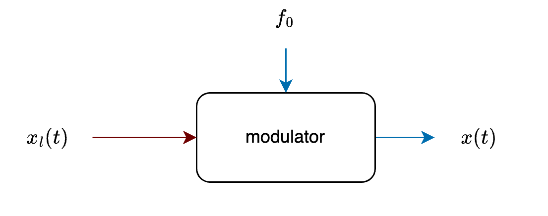
Modulation Process#

The modulation process converts a lowpass signal into a bandpass signal. The system that performs this operation is called a modulator.

Modulator Diagram

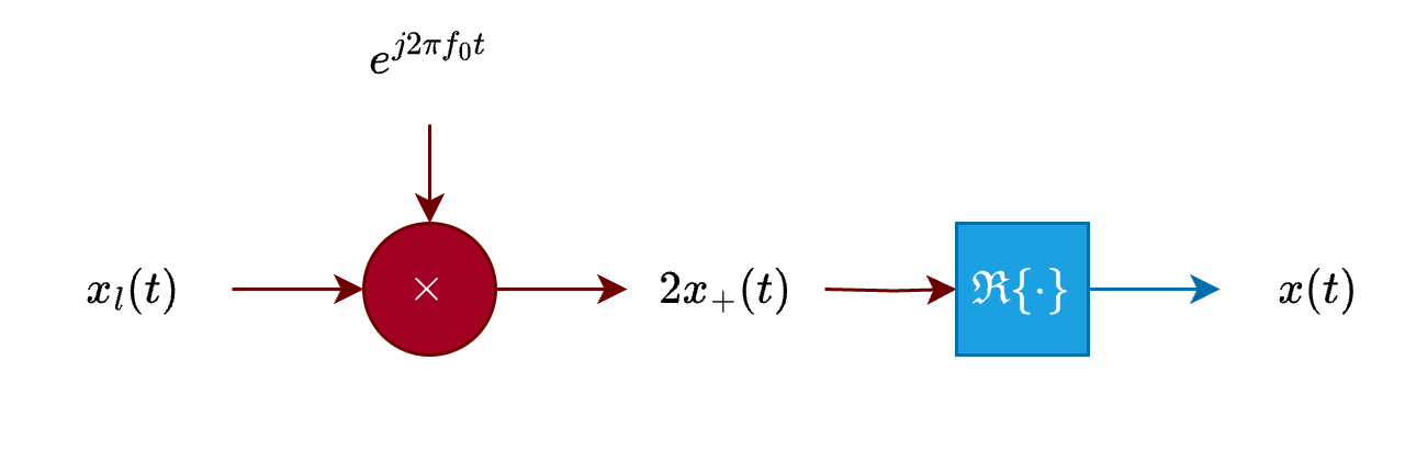
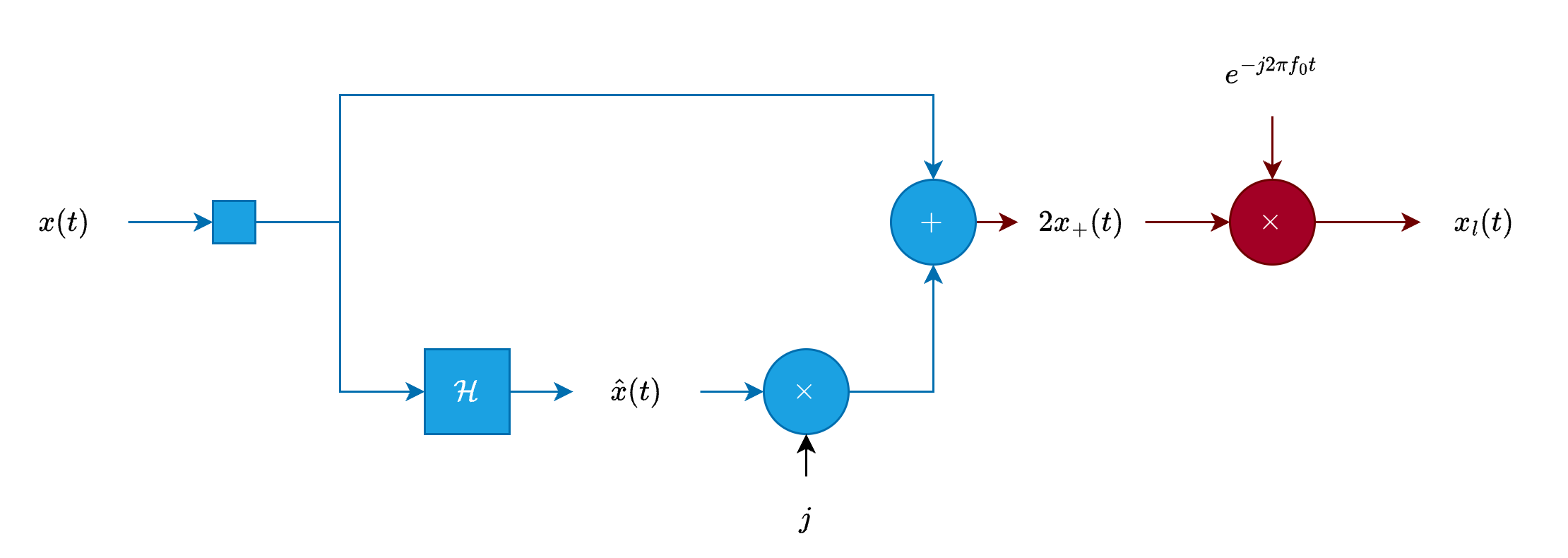
Complex Modulator

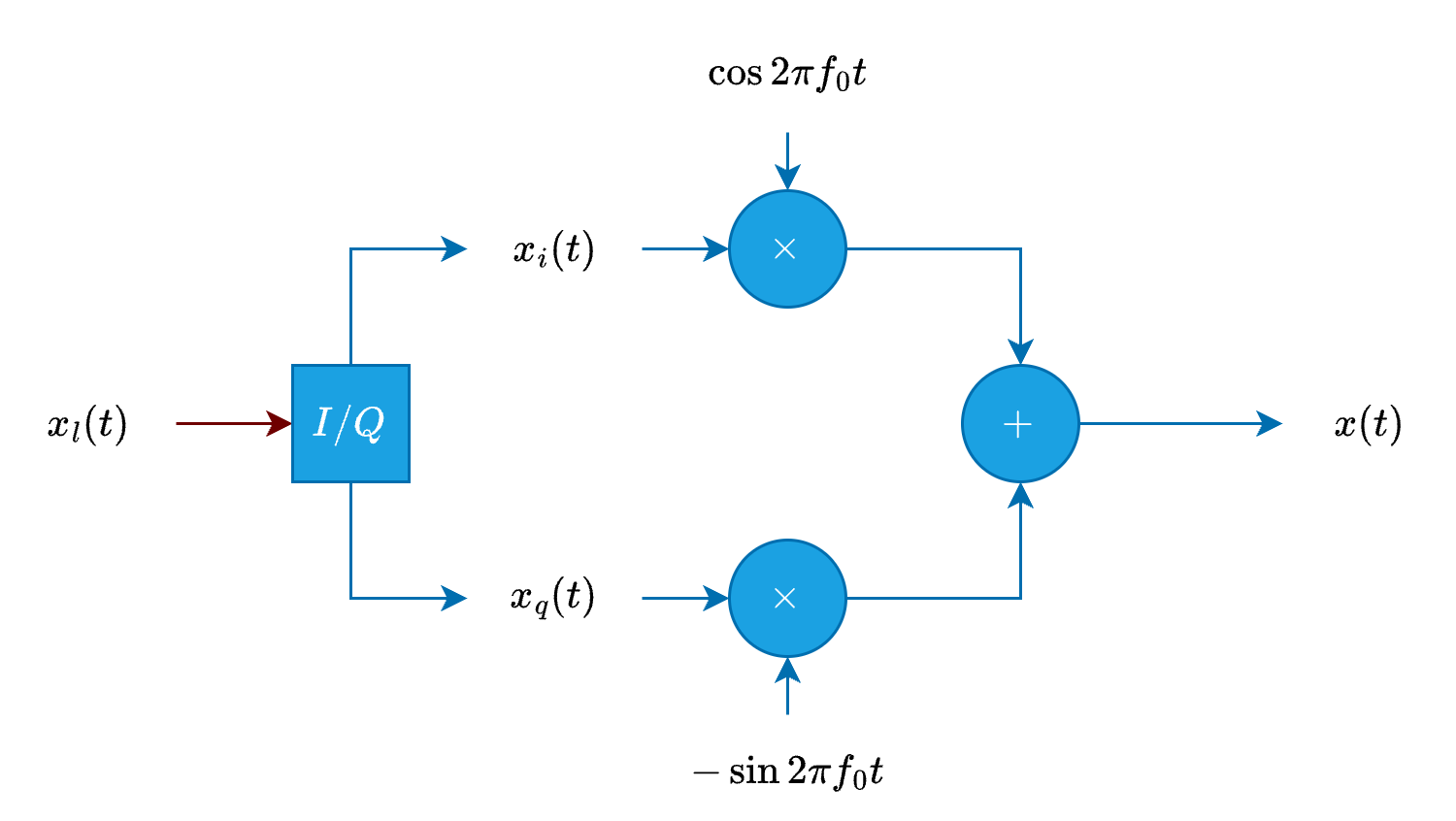
Real Modulator

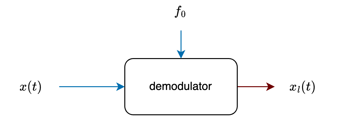
Demodulation Process#

The demodulation process extracts the lowpass signal ($x_l(t)$, or $x_i(t)$ and $x_q(t)$) from the bandpass signal $x(t)$.

Demodulator Diagram

Complex Demodulator

Real Demodulator

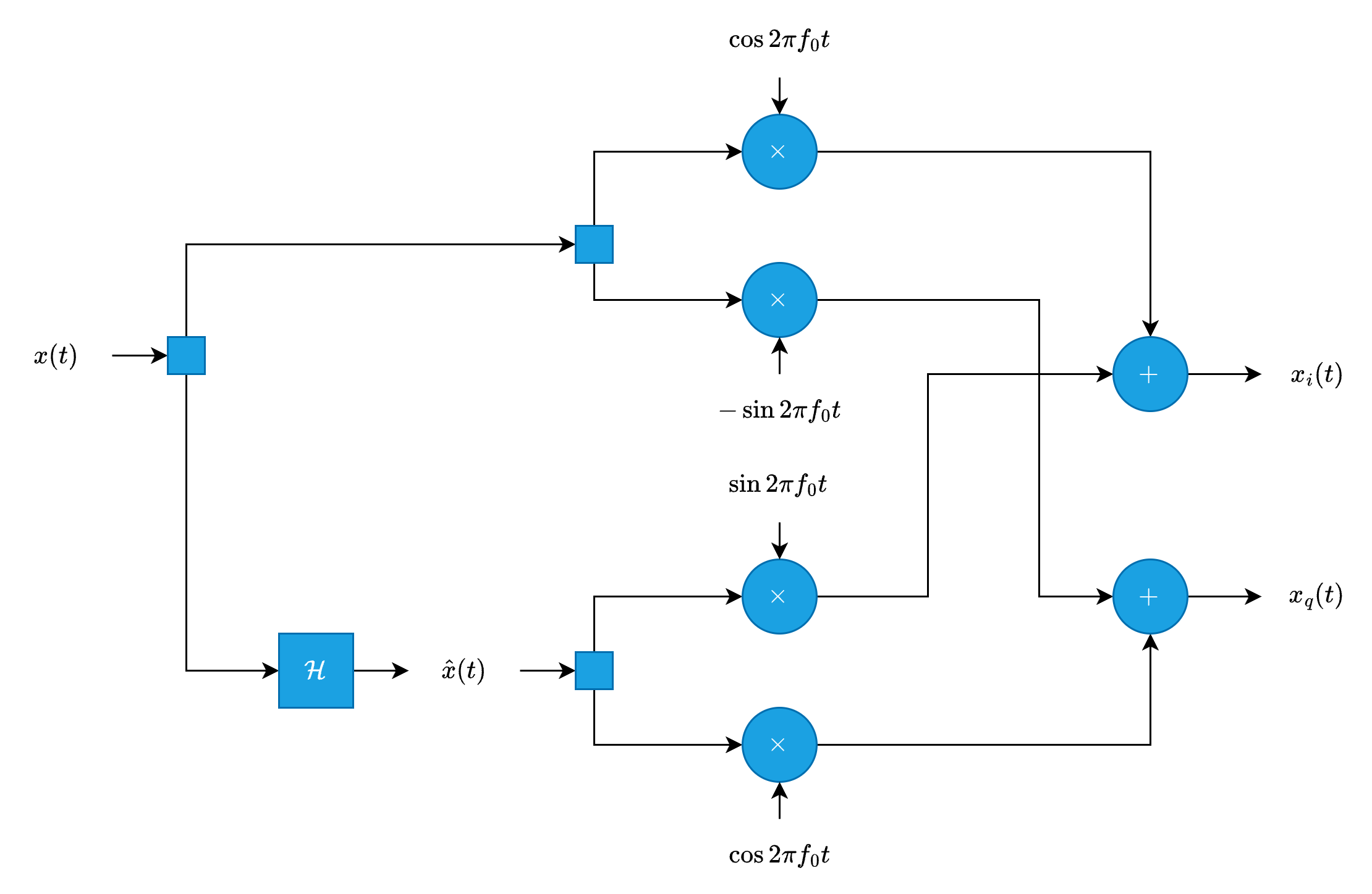
The block labeled $\mathcal{H}$ represents a Hilbert transform, which is an LTI system with:

Impulse response: $h(t) = \frac{1}{\pi t}$
Transfer function: $H(f) = -j\text{sgn}(f)$

Python Example: Bandpass to Lowpass Demodulation#

Bandpass Signal:

\[ x_{\text{bp}}(t) = A \cos(2\pi f_m t) \cdot \cos(2\pi f_0 t) \]

Decomposition into I/Q:

\[ x_i(t), x_q(t) \rightarrow I(t), Q(t) \]

Using the analytic signal and lowpass filtering.

Magnitude and Phase:

\[ r(t), \theta(t) \quad \text{from complex signal} \]

\[ r_{\text{ana}}(t), \theta_{\text{ana}}(t) \quad \text{from I/Q components} \]

Bandpass Signal Generation#

Generate a bandpass signal by modulating a lowpass message signal onto a carrier.

Time Vector:

\[ t = \{0, \frac{1}{f_s}, \frac{2}{f_s}, \ldots, T\} \]

Represents time samples for signal generation.

Lowpass Signal:

\[ x_{\text{lp}}(t) = A \cdot \cos(2\pi f_m t) \]

A cosine wave at message frequency $ f_m $ with amplitude $ A $.

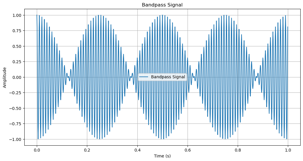
Bandpass Signal:

\[ x_{\text{bp}}(t) = x_{\text{lp}}(t) \cdot \cos(2\pi f_0 t) \]

The lowpass signal is modulated onto a carrier frequency $ f_0 $ to generate a bandpass signal.

import numpy as np
import matplotlib.pyplot as plt

# Define parameters
T = 1                # Signal duration (seconds)
f0 = 100             # Carrier frequency (Hz)
fm = 2               # Message signal frequency (Hz)
fs = 1000            # Sampling frequency (samples per second)
t = np.arange(0, T, 1/fs)  # Time vector (from 0 to T with step size 1/fs)

# Generate a lowpass signal (message signal)
A = 1                # Amplitude of the message signal
x_t_real_lp = A * np.cos(2 * np.pi * fm * t)  # Real-valued lowpass message signal

# Modulate the message signal onto a carrier to create a bandpass signal
x_t_bp = x_t_real_lp * np.cos(2 * np.pi * f0 * t)  # Bandpass signal

# Plot the bandpass signal
plt.figure(figsize=(12, 6))
plt.plot(t, x_t_bp, label='Bandpass Signal')
plt.title('Bandpass Signal')
plt.xlabel('Time (s)')
plt.ylabel('Amplitude')
plt.grid(True)  # Add a grid for better visualization
plt.legend()
plt.show()

_images/b54a5c8606a4aadc27fdb6924d8c7aff74a1268d2690337d7f10cba7d7a17d84.png

Analytic Signal, In-phase, and Quadrature Components#

Decompose a bandpass signal into its analytic signal, in-phase, and quadrature components.

Hilbert Transform (Analytic Signal):

The analytic signal $ \hat{x}(t) $ is: $$ \hat{x}(t) = x_{\text{bp}}(t) + j \cdot H\{x_{\text{bp}}(t)\} $$

where $ H\{\cdot\} $ is the Hilbert transform.

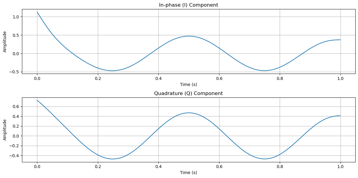
In-phase Component:

Mixing down to baseband involves multiplication by a cosine:

\[ x_i(t) = \Re\left[x_{\text{bp}}(t) \cdot \cos(2\pi f_0 t) + \hat{x}(t) \cdot \sin(2\pi f_0 t)\right] \]

Quadrature Component:

The quadrature component is extracted by:

\[ x_q(t) = \Re\left[\hat{x}(t) \cdot \cos(2\pi f_0 t) - x_{\text{bp}}(t) \cdot \sin(2\pi f_0 t)\right] \]

Lowpass Filtering:

Use a Butterworth lowpass filter to remove high-frequency components:

\[ I(t) = \text{LPF}(x_i(t)), \quad Q(t) = \text{LPF}(x_q(t)) \]

where LPF is the lowpass filtering operation.

Complex Lowpass Equivalent:

Combine the in-phase and quadrature components:

\[ x_{\text{lowpass}}(t) = I(t) + j \cdot Q(t) \]

import numpy as np
import matplotlib.pyplot as plt
from scipy.signal import hilbert, butter, filtfilt

# Generate the analytic signal (complex signal using Hilbert transform)
x_hat = hilbert(x_t_bp)  # Analytic signal of the bandpass signal

# Mix down the analytic signal to baseband
xi_t = np.real(x_t_bp * np.cos(2 * np.pi * f0 * t) + x_hat * np.sin(2 * np.pi * f0 * t))  # In-phase component
xq_t = np.real(x_hat * np.cos(2 * np.pi * f0 * t) - x_t_bp * np.sin(2 * np.pi * f0 * t))  # Quadrature component

# Design a low-pass Butterworth filter to remove high-frequency components
b, a = butter(2, 2 * fm / (fs / 2))  # Butterworth filter of order 2 with cutoff at 2*fm
I = filtfilt(b, a, xi_t)  # Filtered In-phase (I) component
Q = filtfilt(b, a, xq_t)  # Filtered Quadrature (Q) component

# Form the complex lowpass equivalent signal
complex_lowpass_equivalent = I + 1j * Q  # Complex lowpass representation of the signal

# Plot the In-phase (I) and Quadrature (Q) components
plt.figure(figsize=(12, 6))

# Plot the In-phase (I) component
plt.subplot(2, 1, 1)
plt.plot(t, I, linewidth=1.5)
plt.title('In-phase (I) Component')
plt.xlabel('Time (s)')
plt.ylabel('Amplitude')
plt.grid(True)

# Plot the Quadrature (Q) component
plt.subplot(2, 1, 2)
plt.plot(t, Q, linewidth=1.5)
plt.title('Quadrature (Q) Component')
plt.xlabel('Time (s)')
plt.ylabel('Amplitude')
plt.grid(True)

plt.tight_layout()
plt.show()

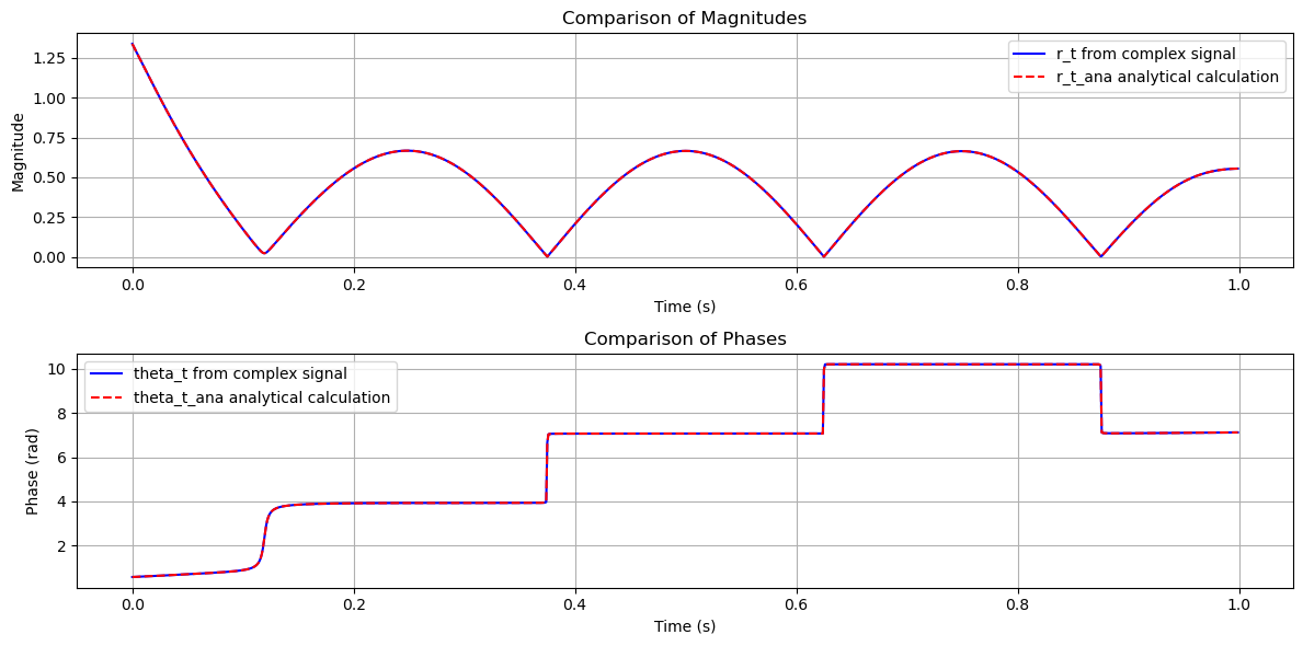
_images/455be70658080560adc00e3eb163bd548428128680f6e15e1ae1fb80844de9fd.png

Magnitude and Phase#

Compute and compare the magnitude and phase of a signal from the complex representation and analytical calculations.

Magnitude from Complex Signal:

\[ r(t) = |x_{\text{lowpass}}(t)| \]

Phase from Complex Signal:

\[ \theta(t) = \angle x_{\text{lowpass}}(t) \]

Analytical Magnitude:

Using $ I(t) $ (in-phase) and $ Q(t) $ (quadrature):

\[ r_{\text{ana}}(t) = \sqrt{I(t)^2 + Q(t)^2} \]

Analytical Phase:

Phase is computed using the arctangent of $ Q(t) $ and $ I(t) $:

\[ \theta_{\text{ana}}(t) = \arctan2(Q(t), I(t)) \]

Comparison:

Compare $ r(t) $ with $ r_{\text{ana}}(t) $, and $ \theta(t) $ with $ \theta_{\text{ana}}(t) $ by plotting.

import numpy as np
import matplotlib.pyplot as plt

# Compute magnitude and phase from the complex lowpass signal
r_t = np.abs(complex_lowpass_equivalent)  # Magnitude of the complex signal
theta_t = np.angle(complex_lowpass_equivalent)  # Phase of the complex signal

# Compute magnitude and phase analytically using filtered I and Q components
r_t_ana = np.sqrt(I**2 + Q**2)  # Analytical magnitude calculation
theta_t_ana = np.arctan2(Q, I)  # Analytical phase calculation using arctangent function

# Plot comparison of magnitudes
plt.figure(figsize=(12, 6))

# Magnitude comparison
plt.subplot(2, 1, 1)
plt.plot(t, r_t, 'b-', linewidth=1.5, label='r_t from complex signal')
plt.plot(t, r_t_ana, 'r--', linewidth=1.5, label='r_t_ana analytical calculation')
plt.title('Comparison of Magnitudes')
plt.xlabel('Time (s)')
plt.ylabel('Magnitude')
plt.legend()
plt.grid(True)

# Phase comparison
plt.subplot(2, 1, 2)
plt.plot(t, np.unwrap(theta_t), 'b-', linewidth=1.5, label='theta_t from complex signal')
plt.plot(t, np.unwrap(theta_t_ana), 'r--', linewidth=1.5, label='theta_t_ana analytical calculation')
plt.title('Comparison of Phases')
plt.xlabel('Time (s)')
plt.ylabel('Phase (rad)')
plt.legend()
plt.grid(True)

# Adjust layout and show the plots
plt.tight_layout()
plt.show()

_images/44a20b382f62ef7f9bacf189cff03e135a2f95f68a634b3b6a9db3695b9257d9.png

Matlab Example: Modulation and Demodulation Using Complex Envelope#

This example demonstrates the step-by-step of a fundamental communication process:

Modulation: Information is encoded into a higher carrier frequency to prepare it for transmission.
Transmission: The modulated signals are sent through a physical channel, which may introduce noise.
Reception: The noisy waveforms are received at the destination.
Demodulation: The received signals are processed to extract and reconstruct the original information.

Modulation and Demodulation Using Complex Envelope