Spectrum

Definition
The Fourier Transform of a signal reveals its spectrum, which provides critical information about the signal’s frequency content. Mathematically, if \(x(t)\) is a time-domain signal, its spectrum is given by \(X(f)\), where:

\[ x(t) \overset{\mathcal{F}}{\longrightarrow} X(f). \]

This spectrum \(X(f)\) quantifies how much of each frequency \(f\) is present in the signal \(x(t)\).

Complex Conjugation and Hermitian Symmetry

The Fourier Transform of the complex conjugate of a signal, \(x^*(t)\), is related to the spectrum by:

\[ \mathcal{F}\{x^*(t)\} = X^*(-f). \]

For real-valued signals \(x(t)\), the spectrum exhibits Hermitian symmetry, where:

\[ X(-f) = X^*(f). \]

This means that the magnitude of the spectrum is symmetric (\(|X(-f)| = |X(f)|\)) and the phase is anti-symmetric (\(\angle X(-f) = -\angle X(f)\)). In other words:

• The magnitude spectrum of a real signal is an even function, symmetric about the vertical axis.

• The phase spectrum of a real signal is an odd function, symmetric about the origin.

Frequency Support

Definition
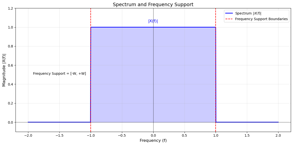
The frequency support of a signal refers to the range of frequencies over which the spectrum \(X(f)\) is non-zero. For band-limited signals, this support is typically defined as:

\[ [-W, +W], \]

where \(W\) is the maximum frequency of the signal’s spectrum.

Positive and Negative Spectrum

The spectrum of a signal can be decomposed into its positive spectrum (\(X_+(f)\)) and negative spectrum (\(X_-(f)\)), which are defined as follows:

\[\begin{split} X_+(f) = \begin{cases} X(f), & f > 0, \\ \frac{1}{2}X(0), & f = 0, \\ 0, & f < 0, \end{cases} \end{split}\]

\[\begin{split} X_-(f) = \begin{cases} X(f), & f < 0, \\ \frac{1}{2}X(0), & f = 0, \\ 0, & f > 0. \end{cases} \end{split}\]

This decomposition separates the spectrum into components that correspond to positive and negative frequencies, facilitating the analysis of complex and real-valued signals.

Python Simulation

import numpy as np
import matplotlib.pyplot as plt

# Define frequency range and spectrum
f = np.linspace(-2, 2, 1000)  # Frequency range from -2W to 2W
spectrum = np.where((f >= -1) & (f <= 1), 1, 0)  # Define spectrum: 1 in [-W, W], 0 otherwise

# Plotting the spectrum and frequency support
plt.figure(figsize=(12, 6))
plt.plot(f, spectrum, label="Spectrum $|X(f)|$", color='blue', lw=2)
plt.axvline(-1, color='red', linestyle='--', label="Frequency Support Boundaries")
plt.axvline(1, color='red', linestyle='--')
plt.fill_between(f, spectrum, color='blue', alpha=0.2)

# Annotate the frequency support region
plt.text(-1.5, 0.5, "Frequency Support = [-W, +W]", fontsize=10, color='black', ha='center')
plt.text(0, 1.05, "|X(f)|", fontsize=12, color='blue', ha='center')

# Customize plot appearance
plt.title("Spectrum and Frequency Support", fontsize=14)
plt.xlabel("Frequency (f)", fontsize=12)
plt.ylabel("Magnitude |X(f)|", fontsize=12)
plt.axhline(0, color='black', linewidth=0.5)
plt.axvline(0, color='black', linewidth=0.5)
plt.grid(alpha=0.3)
plt.legend(fontsize=10)
plt.ylim([-0.1, 1.2])
plt.tight_layout()

# Show plot
plt.show()

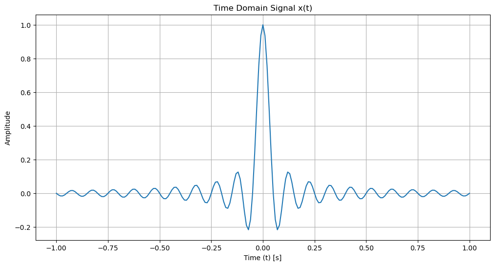
Example of sinc signal

The time-domain sinc signal is defined as:

\[ \text{sinc}(t) = \frac{\sin(2\pi B t)}{2\pi B t}, \]

where \( B \) is the bandwidth.

Fourier Transform of a Sinc Signal

The Fourier Transform (FT) of a signal \( x(t) \) is given by:

\[ X(f) = \int_{-\infty}^{\infty} x(t) e^{-j 2 \pi f t} dt. \]

Substituting \( \text{sinc}(t) \) into this definition:

\[ X(f) = \int_{-\infty}^{\infty} \frac{\sin(2\pi B t)}{2\pi B t} e^{-j 2 \pi f t} dt. \]

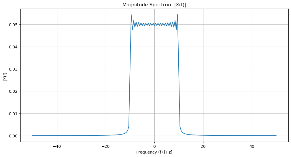
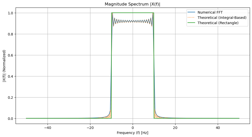
The sinc function in the time domain is known to have a rectangular Fourier Transform:

\[\begin{split} X(f) = \Pi(f) = \begin{cases} 1, & |f| \leq B, \\ 0, & |f| > B. \end{cases} \end{split}\]

This result means that the Fourier Transform of a sinc function is a rectangle function in the frequency domain, centered at \( f = 0 \) with a width of \( 2B \).

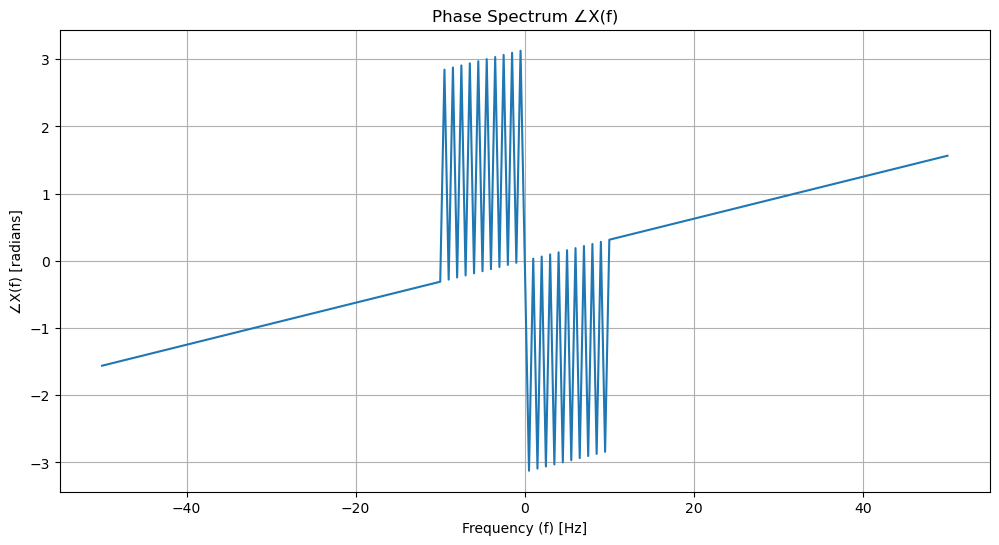
Recall that the magnitude of the spectrum is symmetric (\(|X(-f)| = |X(f)|\)) and the phase is anti-symmetric (\(\angle X(-f) = -\angle X(f)\)):

• The magnitude spectrum of a real signal is an even function, symmetric about the vertical axis.

• The phase spectrum of a real signal is an odd function, symmetric about the origin.

import numpy as np
import matplotlib.pyplot as plt
from scipy.integrate import quad
import warnings
warnings.filterwarnings('ignore')

# Define the duration of the sinc signal
T = 1  # seconds

# Define the time domain parameters
fs = 100  # Sampling frequency in Hz
t = np.arange(-T, T + 1/fs, 1/fs)  # Time vector
dt = T/fs  # Time step size

# Define the sinc function in the time domain
bandwidth = 10  # Bandwidth of the lowpass signal
x_t = np.sinc(2 * bandwidth * t)  # sinc in numpy is normalized by pi

# Perform the numerical Fourier Transform using the FFT
X_f_sim = np.fft.fftshift(np.fft.fft(x_t)) * dt  # Multiply by dt to approximate the integral

# Generate the frequency vector for the numerical approach
f_num = np.linspace(-fs/2, fs/2, len(X_f_sim))

# Plot the time-domain sinc signal
plt.figure(figsize=(12, 6))
plt.plot(t, x_t, linewidth=1.5)
plt.title('Time Domain Signal x(t)')
plt.xlabel('Time (t) [s]')
plt.ylabel('Amplitude')
plt.grid(True)

# Calculate magnitude and phase of the numerical Fourier Transform
magnitude = np.abs(X_f_sim)
phase = np.angle(X_f_sim)

# Plot the magnitude spectrum
plt.figure(figsize=(12, 6))
plt.plot(f_num, magnitude, linewidth=1.5)
plt.title('Magnitude Spectrum |X(f)|')
plt.xlabel('Frequency (f) [Hz]')
plt.ylabel('|X(f)|')
plt.grid(True)

# Plot the phase spectrum
plt.figure(figsize=(12, 6))
plt.plot(f_num, phase, linewidth=1.5)
plt.title('Phase Spectrum ∠X(f)')
plt.xlabel('Frequency (f) [Hz]')
plt.ylabel('∠X(f) [radians]')
plt.grid(True)

plt.show()

# Define the frequency range for the theoretical FT calculation
f_theo = np.linspace(-fs/2, fs/2, 1024)  # More points for smoother theoretical curve

# Pre-allocate the array for the theoretical FT
X_f_theo = np.zeros_like(f_theo, dtype=complex)

# Calculation limits: choose a limit that contains most of the sinc function energy
integration_limit = 10 / bandwidth  # 10 cycles of the sinc function

# Calculate the theoretical Fourier Transform using numerical integration
for k, f_k in enumerate(f_theo):
    integral_func = lambda t: np.sinc(2 * bandwidth * t) * np.exp(-1j * 2 * np.pi * f_k * t)
    X_f_theo[k], _ = quad(integral_func, -integration_limit, integration_limit)

# Normalize the numerical and theoretical FT for comparison
X_f_sim_norm = np.abs(X_f_sim) / np.max(np.abs(X_f_sim))
X_f_theo_norm = np.abs(X_f_theo) / np.max(np.abs(X_f_theo))

# Calculate the theoretical FT for the sinc function (rectangle function)
f_theo_rect = np.linspace(-fs/2, fs/2, 1024)
X_f_theo_rect = np.where(np.abs(f_theo_rect) <= bandwidth, 1, 0)

# Combine all three curves into one plot
plt.figure(figsize=(12, 6))
plt.plot(f_num, X_f_sim_norm, label='Numerical FFT', linewidth=1.5)
plt.plot(f_theo, X_f_theo_norm, label='Theoretical (Integral-Based)', linestyle='dotted', linewidth=1.5)
plt.plot(f_theo_rect, X_f_theo_rect, label='Theoretical (Rectangle)', linewidth=1.5)
plt.title('Magnitude Spectrum |X(f)|')
plt.xlabel('Frequency (f) [Hz]')
plt.ylabel('|X(f)| (Normalized)')
plt.legend()  # Add legend to distinguish the curves
plt.grid(True)
plt.show()

Matlab Example: Compute Signal Spectrum

Compute Signal Spectrum Using Different Windows

Open the Signal Analyzer App

• Using MATLAB Toolstrip: On the APPS tab, click the signal Analyzer app icon

• Using MATLAB command prompt: Enter signalAnalyzer