Rayleigh Random Variable#
Consider two independent and identically distributed (iid) Gaussian random variables, denoted as \( X_1 \) and \( X_2 \), each following a normal distribution with mean zero and variance \( \sigma^2 \), i.e.,
The random variable \( X \), defined as
follows a Rayleigh distribution.
Probability Density Function (PDF)#
The probability density function (PDF) of a Rayleigh-distributed random variable is given by
In the Rayleigh probability density function (PDF), the parameter \( \sigma \) is known as the scale parameter. It determines the spread of the distribution and affects both the peak and tail behavior of the PDF.
Mathematically, in the Rayleigh PDF given above, \( \sigma \) controls the dispersion of the distribution.
Expected Value and Variance#
The expected value and variance of \( X \) are given by
Cumulative Distribution Function (CDF)#
The cumulative distribution function (CDF) of a Rayleigh-distributed random variable is expressed as
import numpy as np
import matplotlib.pyplot as plt
from scipy.stats import rayleigh
# Set parameters
sigma = 1 # Standard deviation of Gaussian variables
num_samples = 100000 # Number of samples
# Generate Rayleigh RV from two Gaussian RVs
X1 = np.random.normal(0, sigma, num_samples)
X2 = np.random.normal(0, sigma, num_samples)
rayleigh_simulated = np.sqrt(X1**2 + X2**2)
# Generate Rayleigh RV using built-in function
rayleigh_builtin = rayleigh.rvs(scale=sigma, size=num_samples)
# Define bins for histogram
bins = np.linspace(0, np.max(rayleigh_simulated), 100)
# Compute theoretical PDF
x_vals = np.linspace(0, np.max(rayleigh_simulated), 1000)
theoretical_pdf = (x_vals / sigma**2) * np.exp(-x_vals**2 / (2 * sigma**2))
# Plot the results
plt.figure(figsize=(8, 6))
# Histogram for numerically estimated PDFs
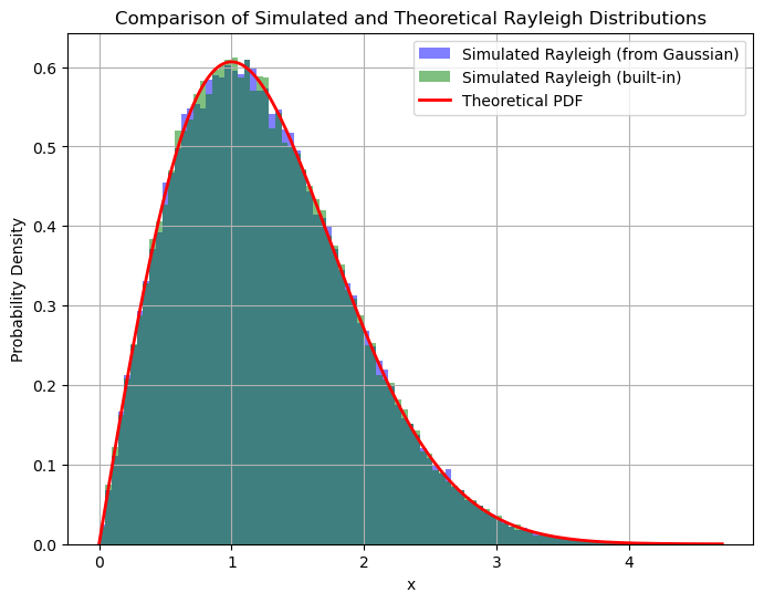
plt.hist(rayleigh_simulated, bins, density=True, alpha=0.5, label="Simulated Rayleigh (from Gaussian)", color='blue')
plt.hist(rayleigh_builtin, bins, density=True, alpha=0.5, label="Simulated Rayleigh (built-in)", color='green')
# Plot theoretical PDF
plt.plot(x_vals, theoretical_pdf, 'r-', linewidth=2, label="Theoretical PDF")
# Labels and title
plt.xlabel("x")
plt.ylabel("Probability Density")
plt.title("Comparison of Simulated and Theoretical Rayleigh Distributions")
plt.legend()
plt.grid(True)
# Show plot
plt.show()
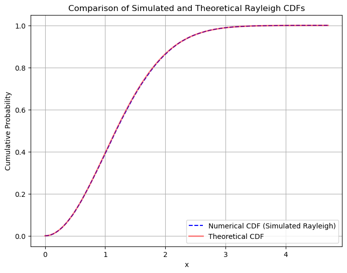
# Compute numerical CDF from simulated Rayleigh (from Gaussian)
sorted_rayleigh_simulated = np.sort(rayleigh_simulated)
num_cdf = np.arange(1, num_samples + 1) / num_samples

# Compute theoretical CDF
theoretical_cdf = 1 - np.exp(-x_vals**2 / (2 * sigma**2))

# Plot the results
plt.figure(figsize=(8, 6))

# Plot numerical CDF as a histogram
plt.plot(sorted_rayleigh_simulated, num_cdf, label="Numerical CDF (Simulated Rayleigh)", color='blue', linestyle='--')

# Plot theoretical CDF
plt.plot(x_vals, theoretical_cdf, label="Theoretical CDF", color='red', linewidth=2, alpha=0.5)

# Labels and title
plt.xlabel("x")
plt.ylabel("Cumulative Probability")
plt.title("Comparison of Simulated and Theoretical Rayleigh CDFs")
plt.legend()
plt.grid(True)

# Show plot
plt.show()
# Compute numerical mean and variance from simulated Rayleigh (from Gaussian)
numerical_mean = np.mean(rayleigh_simulated)
numerical_variance = np.var(rayleigh_simulated)

# Compute theoretical mean and variance based on given expressions
theoretical_mean = sigma * np.sqrt(np.pi / 2)
theoretical_variance = (2 - np.pi / 2) * sigma**2

# Create a DataFrame for display
data = {
    "Statistic": ["Mean", "Variance"],
    "Numerical (Simulated)": [numerical_mean, numerical_variance],
    "Theoretical": [theoretical_mean, theoretical_variance]
}

df = pd.DataFrame(data)

# Display the DataFrame
print(df)
  Statistic  Numerical (Simulated)  Theoretical
0      Mean               1.257428     1.253314
1  Variance               0.430243     0.429204
Illustrate the impact of the parameter \(\sigma\)#
# Define different sigma values to analyze their impact
sigma_values = [0.5, 1, 2]

# Set number of samples
num_samples = 100000

# Define x-values for theoretical PDFs and CDFs
x_vals = np.linspace(0, 5, 1000)

# Create a figure for PDF comparison
plt.figure(figsize=(8, 6))

for sigma in sigma_values:
    # Simulate Rayleigh from Gaussian for different sigma values
    X1 = np.random.normal(0, sigma, num_samples)
    X2 = np.random.normal(0, sigma, num_samples)
    rayleigh_simulated = np.sqrt(X1**2 + X2**2)

    # Compute histogram for numerical PDF
    hist_vals, bins = np.histogram(rayleigh_simulated, bins=100, density=True)
    bin_centers = (bins[:-1] + bins[1:]) / 2

    # Compute theoretical PDF
    theoretical_pdf = (x_vals / sigma**2) * np.exp(-x_vals**2 / (2 * sigma**2))

    # Plot numerical PDF
    plt.plot(bin_centers, hist_vals, linestyle='dashed', label=f"Numerical PDF (σ={sigma})")

    # Plot theoretical PDF
    plt.plot(x_vals, theoretical_pdf, linewidth=2, label=f"Theoretical PDF (σ={sigma})", alpha=0.5)

# Labels and legend
plt.xlabel("x")
plt.ylabel("Probability Density")
plt.title("Impact of σ on Rayleigh PDF")
plt.legend()
plt.grid(True)
plt.show()
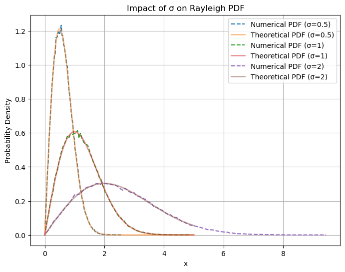
A larger \( \sigma \) results in a wider spread, shifting the peak of the distribution to the right, while a smaller \( \sigma \) makes the distribution more concentrated around smaller \( x \)-values.
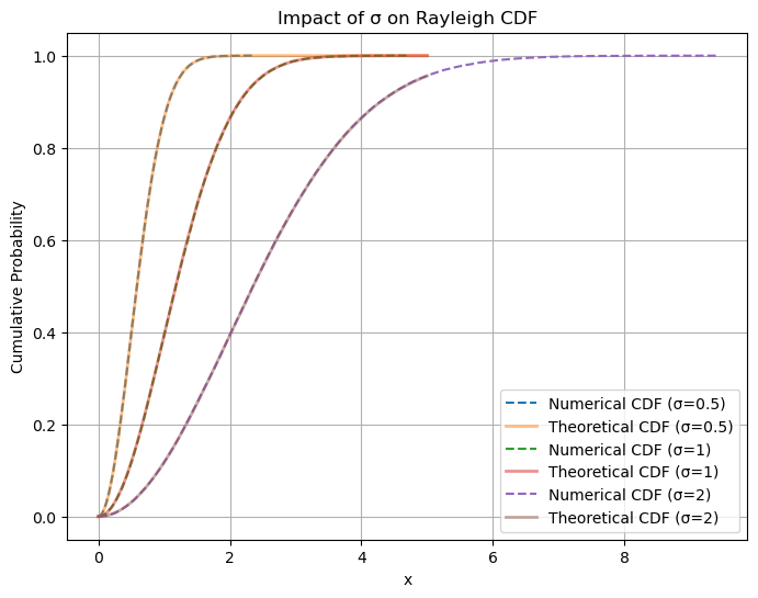
# Create a figure for CDF comparison
plt.figure(figsize=(8, 6))

for sigma in sigma_values:
    # Simulate Rayleigh from Gaussian for different sigma values
    X1 = np.random.normal(0, sigma, num_samples)
    X2 = np.random.normal(0, sigma, num_samples)
    rayleigh_simulated = np.sqrt(X1**2 + X2**2)

    # Compute empirical CDF
    sorted_rayleigh_simulated = np.sort(rayleigh_simulated)
    num_cdf = np.arange(1, num_samples + 1) / num_samples

    # Compute theoretical CDF
    theoretical_cdf = 1 - np.exp(-x_vals**2 / (2 * sigma**2))

    # Plot numerical CDF
    plt.plot(sorted_rayleigh_simulated, num_cdf, linestyle='dashed', label=f"Numerical CDF (σ={sigma})")

    # Plot theoretical CDF
    plt.plot(x_vals, theoretical_cdf, linewidth=2, label=f"Theoretical CDF (σ={sigma})", alpha=0.5)

# Labels and legend
plt.xlabel("x")
plt.ylabel("Cumulative Probability")
plt.title("Impact of σ on Rayleigh CDF")
plt.legend()
plt.grid(True)
plt.show()