Filter, Channel, and System

Lowpass Equivalent of a Bandpass System

Bandpass Systems

A bandpass system is a system whose transfer function is centered around a frequency \(f_0\) and its mirror image at \(-f_0\).

Definition: Lowpass Equivalent of System Impulse Response
A bandpass system is characterized by an impulse response \(h(t)\), which is itself a bandpass signal.
The lowpass equivalent of \(h(t)\), denoted by \(h_l(t)\), is defined as:

\[ h(t) = \Re \big\{ h_l(t)e^{j2\pi f_0t} \big\} \]

Input-Output Relationship in Bandpass Systems

When a bandpass signal \(x(t)\) passes through a bandpass system with impulse response \(h(t)\), the output \(y(t)\) is also a bandpass signal. The relationship between the spectra of the input and output is:

\[ Y(f) = X(f)H(f) \]

Lowpass Equivalent Relationship

For the lowpass equivalents of the signals and system, the relationship is given by:

\[ Y_l(f) = 2Y(f + f_0)u_{-1}(f + f_0) \]

Expanding this:

\[ Y_l(f) = 2X(f + f_0)H(f + f_0)u_{-1}(f + f_0) \]

Simplifying further:

\[ \boxed{ Y_l(f) = \frac{1}{2} X_l(f)H_l(f) } \]

Time Domain Relation

In the time domain, the relation between the input \(x(t)\), the system impulse response \(h(t)\), and the output \(y(t)\) is:

\[ \boxed{ y(t) = \frac{1}{2} x(t) \circledast h_l(t) } \]

where \(\circledast\) denotes the convolution.

Key Insight

• When a bandpass signal passes through a bandpass system, the relationship between their lowpass equivalents is analogous to that between the bandpass signals.

• The only difference is the introduction of a scaling factor of \(\frac{1}{2}\) for the lowpass equivalents.

Matlab Example: Lowpass Filtering of Tones

Reference: Lowpass Filtering of Tones

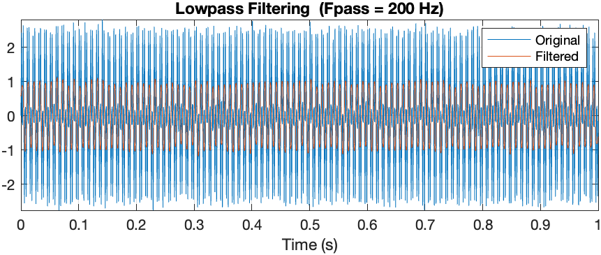
This example demonstrates how to generate, process, and analyze a signal with specific frequency components and noise, and how a lowpass filter isolates desired frequencies:

Signal Generation:

• A signal is created with a duration of 1 second, sampled at a rate of 1 kHz (1000 samples per second). This means the signal will have 1000 samples for the 1-second duration.

• The signal consists of two sinusoidal tones:

  • A low-frequency tone at 100 Hz.

  • A high-frequency tone at 300 Hz.

• Amplitude adjustment: The amplitude of the 300 Hz tone is set to twice that of the 100 Hz tone, making it more prominent in the signal.

• Noise addition: Gaussian white noise with a variance of \( \frac{1}{100} \) is added to simulate a realistic noisy environment. White noise introduces random variations across all frequencies.

Lowpass Filtering:

• A lowpass filter is applied to the signal. This filter is designed to pass frequencies below a certain threshold and attenuate higher frequencies.

• The threshold (passband frequency) is set to 200 Hz, meaning:

  • The low-frequency component at 100 Hz is retained.

  • The high-frequency component at 300 Hz is attenuated or removed, along with any noise above 200 Hz.

Matlab Simulation

% Sampling frequency (1 kHz)
fs = 1e3;

% Time vector (1 second duration, sampled at 1 kHz)
t = 0:1/fs:1;

% Generate the signal:
% - Two sinusoidal tones: 100 Hz and 300 Hz
% - Amplitudes are 1 and 2, respectively
% - Add Gaussian white noise with variance 1/100
x = [1 2]*sin(2*pi*[100 300]'.*t) + randn(size(t))/10;

% Apply a lowpass filter:
% - Passband frequency: 200 Hz
% - Sampling frequency: fs (1 kHz)
filtered_x = lowpass(x, 200, fs);

% Plot time-domain and frequency-domain views

3. Visualization:

   • The original signal is displayed in the time domain, showing the combined tones and noise.

   • The filtered signal is displayed to show how the high-frequency tone and noise are reduced, leaving mostly the 100 Hz tone.

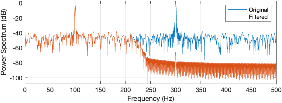
   • Spectra (frequency-domain representations) of both signals are plotted:

     • The spectrum of the original signal shows two peaks at 100 Hz and 300 Hz, corresponding to the tones, along with the noise spread across all frequencies.

     • The spectrum of the filtered signal shows only the peak at 100 Hz, as the 300 Hz tone and higher-frequency noise are removed by the filter.