Gram-Schmidt Procedure for Signals

Given a set of finite-energy signals \( \{s_m(t), m = 1, 2, ..., M\} \), the Gram-Schmidt orthogonalization procedure is used to construct an orthonormal set of waveforms.

Initial Step: Normalize the First Signal

Starting with the first signal \( s_1(t) \), with energy \( E_1 \):

\[ \phi_1(t) = \frac{s_1(t)}{\sqrt{E_1}} \]

This creates the first orthonormal waveform \( \phi_1(t) \), which is \( s_1(t) \) normalized to unit energy.

The Next Step: Orthogonalize the Second Signal

For the second signal \( s_2(t) \), compute its projection onto \( \phi_1(t) \):

\[ c_{21} = \langle s_2(t), \phi_1(t) \rangle = \int_{-\infty}^{\infty} s_2(t) \phi_1^*(t) \, dt \]

Subtract this projection to create a signal orthogonal to \( \phi_1(t) \):

\[ \gamma_2(t) = s_2(t) - c_{21} \phi_1(t) \]

Normalize \( \gamma_2(t) \) to obtain the second orthonormal waveform:

\[ \phi_2(t) = \frac{\gamma_2(t)}{\sqrt{E_2}} \]

where \( E_2 = \int_{-\infty}^{\infty} |\gamma_2(t)|^2 dt \) is the energy of \( \gamma_2(t) \).

A General Step: Orthogonalization of the \( k \)-th Signal

For the \( k \)-th signal \( s_k(t) \), compute:

\[ \gamma_k(t) = s_k(t) - \sum_{i=1}^{k-1} c_{ki} \phi_i(t) \]

where:

\[ c_{ki} = \langle s_k(t), \phi_i(t) \rangle = \int_{-\infty}^{\infty} s_k(t) \phi_i^*(t) \, dt \]

Normalize \( \gamma_k(t) \) to obtain the \( k \)-th orthonormal waveform:

\[ \phi_k(t) = \frac{\gamma_k(t)}{\sqrt{E_k}} \]

where \( E_k = \int_{-\infty}^{\infty} |\gamma_k(t)|^2 dt \).

Resultant Orthogonal Set of Waveforms
This process continues for all \( M \) signals \( \{s_m(t)\} \), resulting in \( N \leq M \) orthonormal waveforms. These waveforms span the signal space defined by the original set.

Example: Applying the Gram-Schmidt Procedure to Rectangular Signals

We apply the Gram-Schmidt process to four rectangular signals \( s_1(t), s_2(t), s_3(t), \) and \( s_4(t) \), where:

\( s_1(t) = \begin{cases} 1, & 0 \leq t \leq 2 \\ 0, & \text{otherwise} \end{cases} \)

\( s_2(t) = \begin{cases} 1, & 0 \leq t \leq 1 \\ -1, & 1 < t \leq 2 \\ 0, & \text{otherwise} \end{cases} \)

\( s_3(t) = \begin{cases} 1, & 0 \leq t \leq 2 \\ -1, & 2 < t \leq 3 \\ 0, & \text{otherwise} \end{cases} \)

\( s_4(t) = \begin{cases} -1, & 0 \leq t \leq 3 \\ 0, & \text{otherwise} \end{cases} \)

import numpy as np
import matplotlib.pyplot as plt

# Define time range
t = np.linspace(0, 3, 1000)

# Define the given signals
s1 = np.where((t >= 0) & (t <= 2), 1, 0)
s2 = np.where((t >= 0) & (t <= 1), 1, np.where((t > 1) & (t <= 2), -1, 0))
s3 = np.where((t >= 0) & (t <= 2), 1, np.where((t > 2) & (t <= 3), -1, 0))
s4 = np.where((t >= 0) & (t <= 3), -1, 0)

# Plot original signals
plt.figure(figsize=(12, 6))

plt.subplot(4, 1, 1)
plt.plot(t, s1, label="s1(t)", color="blue")
plt.title("Signal s1(t)")
plt.grid()

plt.subplot(4, 1, 2)
plt.plot(t, s2, label="s2(t)", color="orange")
plt.title("Signal s2(t)")
plt.grid()

plt.subplot(4, 1, 3)
plt.plot(t, s3, label="s3(t)", color="green")
plt.title("Signal s3(t)")
plt.grid()

plt.subplot(4, 1, 4)
plt.plot(t, s4, label="s4(t)", color="red")
plt.title("Signal s4(t)")
plt.grid()

plt.tight_layout()
plt.show()

Gram-Schmidt Procedure

Step 1: Normalize \( s_1(t) \)

The energy of \( s_1(t) \) is:

\[ E_1 = \int_0^2 1^2 \, dt = 2 \]

The first orthonormal waveform is:

\[ \phi_1(t) = \frac{1}{\sqrt{2}} s_1(t) \]

Step 2: Orthogonalize \( s_2(t) \)

The projection coefficient \( c_{21} \) is:

\[ c_{21} = \langle s_2(t), \phi_1(t) \rangle = \int_0^2 s_2(t) \cdot \frac{1}{\sqrt{2}} \, dt = 0 \]

Since \( c_{21} = 0 \), \( s_2(t) \) and \( \phi_1(t) \) are orthogonal. The energy of \( s_2(t) \) is:

\[ E_2 = \int_0^1 1^2 \, dt + \int_1^2 (-1)^2 \, dt = 1 + 1 = 2 \]

The normalized second orthonormal waveform is:

\[ \phi_2(t) = \frac{1}{\sqrt{2}} s_2(t) \]

Step 3: Orthogonalize \( s_3(t) \)

The projection coefficients are:

\[ c_{31} = \langle s_3(t), \phi_1(t) \rangle = \int_0^2 s_3(t) \cdot \frac{1}{\sqrt{2}} \, dt = \sqrt{2} \]

\[ c_{32} = \langle s_3(t), \phi_2(t) \rangle = \int_0^2 s_3(t) \cdot \frac{1}{\sqrt{2}} \, dt = 0 \]

The residual signal is:

\[\begin{split} \gamma_3(t) = s_3(t) - c_{31} \phi_1(t) = \begin{cases} -1 & \text{if } 2 \leq t < 3 \\ 0 & \text{otherwise} \end{cases} \end{split}\]

The energy of \( \gamma_3(t) \) is:

\[ E_3 = \int_2^3 (-1)^2 \, dt = 1 \]

The normalized third orthonormal waveform is:

\[ \phi_3(t) = \gamma_3(t) \]

Step 4: Orthogonalize \( s_4(t) \)

The projection coefficients are:

\[ c_{41} = \langle s_4(t), \phi_1(t) \rangle = -\sqrt{2}, \quad c_{42} = \langle s_4(t), \phi_2(t) \rangle = 0, \quad c_{43} = \langle s_4(t), \phi_3(t) \rangle = 1 \]

The residual signal is:

\[ \gamma_4(t) = s_4(t) + c_{41} \phi_1(t) + c_{43} \phi_3(t) = 0 \]

Since \( \gamma_4(t) = 0 \), \( s_4(t) \) is a linear combination of \( \phi_1(t) \) and \( \phi_3(t) \). Thus:

\[ \phi_4(t) = 0 \]

Final Results

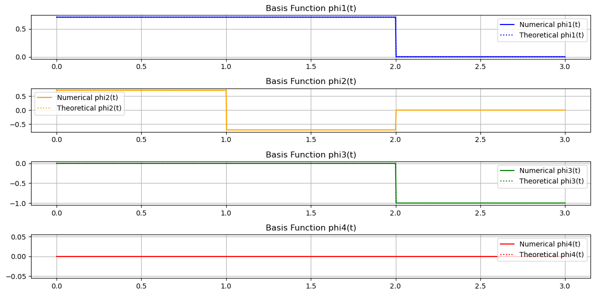
\( \phi_1(t) = \frac{1}{\sqrt{2}} s_1(t) \)

\( \phi_2(t) = \frac{1}{\sqrt{2}} s_2(t) \)

\( \phi_3(t) = \gamma_3(t) = \begin{cases} -1 & \text{if } 2 \leq t < 3 \\ 0 & \text{otherwise} \end{cases} \)

\( \phi_4(t) = 0 \)

The final solution in the form of case functions:

\( \phi_1(t) \) (Normalized \( s_1(t) \)):

\[\begin{split} \phi_1(t) = \begin{cases} \frac{1}{\sqrt{2}} & 0 \leq t \leq 2 \\ 0 & \text{otherwise} \end{cases} \end{split}\]

\( \phi_2(t) \) (Normalized \( s_2(t) \)):

\[\begin{split} \phi_2(t) = \begin{cases} \frac{1}{\sqrt{2}} & 0 \leq t \leq 1 \\ -\frac{1}{\sqrt{2}} & 1 < t \leq 2 \\ 0 & \text{otherwise} \end{cases} \end{split}\]

\( \phi_3(t) \) (Orthogonalized \( s_3(t) \)):

\[\begin{split} \phi_3(t) = \begin{cases} 0 & 0 \leq t \leq 2 \\ -1 & 2 < t \leq 3 \\ 0 & \text{otherwise} \end{cases} \end{split}\]

\( \phi_4(t) \) (Resulting residual signal from \( s_4(t) \)):

\[ \phi_4(t) = 0 \]

# Step-by-step calculation of orthonormal waveforms
phi1 = s1 / np.sqrt(np.trapz(s1**2, t))  # Normalize s1(t)
c21 = np.trapz(s2 * phi1, t)
gamma2 = s2 - c21 * phi1
phi2 = gamma2 / np.sqrt(np.trapz(gamma2**2, t))  # Normalize gamma2

c31 = np.trapz(s3 * phi1, t)
c32 = np.trapz(s3 * phi2, t)
gamma3 = s3 - c31 * phi1 - c32 * phi2
phi3 = gamma3 / np.sqrt(np.trapz(gamma3**2, t))  # Normalize gamma3

c41 = np.trapz(s4 * phi1, t)
c42 = np.trapz(s4 * phi2, t)
c43 = np.trapz(s4 * phi3, t)

gamma4 = s4 - c41 * phi1 - c42 * phi2 - c43 * phi3

# Tolerance threshold for gamma4
tolerance = 1e-6

# Recalculate gamma4 with the threshold applied
if np.sqrt(np.trapz(gamma4**2, t)) < tolerance:
    phi4 = np.zeros_like(t)
else:
    phi4 = gamma4 / np.sqrt(np.trapz(gamma4**2, t))

# Define theoretical results
phi1_theoretical = np.where((t >= 0) & (t <= 2), 1/np.sqrt(2), 0)
phi2_theoretical = np.where((t >= 0) & (t <= 1), 1/np.sqrt(2), np.where((t > 1) & (t <= 2), -1/np.sqrt(2), 0))
phi3_theoretical = np.where((t > 2) & (t <= 3), -1, 0)
phi4_theoretical = np.zeros_like(t)

# Plot basis functions
plt.figure(figsize=(12, 6))

plt.subplot(4, 1, 1)
plt.plot(t, phi1, label="Numerical phi1(t)", color="blue")
plt.plot(t, phi1_theoretical, label="Theoretical phi1(t)", linestyle=":", color="blue")
plt.title("Basis Function phi1(t)")
plt.legend()
plt.grid()

plt.subplot(4, 1, 2)
plt.plot(t, phi2, label="Numerical phi2(t)", color="orange")
plt.plot(t, phi2_theoretical, label="Theoretical phi2(t)", linestyle=":", color="orange")
plt.title("Basis Function phi2(t)")
plt.legend()
plt.grid()

plt.subplot(4, 1, 3)
plt.plot(t, phi3, label="Numerical phi3(t)", color="green")
plt.plot(t, phi3_theoretical, label="Theoretical phi3(t)", linestyle=":", color="green")
plt.title("Basis Function phi3(t)")
plt.legend()
plt.grid()

plt.subplot(4, 1, 4)
plt.plot(t, phi4, label="Numerical phi4(t)", color="red")
plt.plot(t, phi4_theoretical, label="Theoretical phi4(t)", linestyle=":", color="red")
plt.title("Basis Function phi4(t)")
plt.legend()
plt.grid()

plt.tight_layout()
plt.show()

DISCUSSION

Why \( \phi_4(t) \) is Zero: Linear Dependence Explained

During the orthogonalization of \( s_4(t) \) against the orthonormal set \( \{\phi_1(t), \phi_2(t), \phi_3(t)\} \), \( \phi_4(t) \) was found to be zero (or effectively zero within numerical precision). This reflects the linear dependence among the signals.

Linear Dependence Overview:

• A set of functions is linearly dependent if one function can be expressed as a linear combination of others.

• If \( s_4(t) \) is a combination of \( s_1(t), s_2(t), \) and \( s_3(t) \), it does not contribute a new dimension to the signal space.

In the Gram-Schmidt Process:

• The span of \( \{s_1(t), s_2(t), s_3(t)\} \) includes \( s_4(t) \), meaning \( s_4(t) \) is redundant.

• Orthogonalizing \( s_4(t) \) yields \( \phi_4(t) = 0 \) because it lies within the span of the existing orthonormal functions.

Conclusion: Only \( \{\phi_1(t), \phi_2(t), \phi_3(t)\} \) form the orthonormal basis, as \( \phi_4(t) \) does not contribute additional information.