Parameter Estimation#
The set of observables or measurements \( \mathbf{y}_1, \ldots, \mathbf{y}_m \) will be represented in vector notation by \(\vec{\mathbf{y}} = \{\mathbf{y}_1, \ldots, \mathbf{y}_m\}\).
Embedded within the observables are a set of parameters \( \alpha_1, \ldots, \alpha_k \) represented by the parameter vector \(\vec{\alpha} = \{\alpha_1, \ldots, \alpha_k\}\).
The parameter vector refers to the set of parameters to be estimated; it does not refer to the received signal amplitude
The parameter estimation problem is to find a parameter estimate vector \(\vec{\hat{\boldsymbol{\alpha}}}(\vec{\mathbf{y}})\) that depends on the observables.
In vector representation, it is expressed as
Note that the observables vector given later is suppressed in \(\vec{\hat{\alpha}}\) for simplicity, i.e., \( \vec{\hat{\boldsymbol{\alpha}}}(\vec{\mathbf{y}}) \equiv \vec{\hat{\boldsymbol{\alpha}}}.\)
Parameter Estimation Problem#
The parameter estimate \(\vec{\hat{\boldsymbol{\alpha}}}(\vec{\mathbf{y}})\) depends on the random observables and is therefore itself a random variable (or random vector).
The parameter \(\vec{\boldsymbol{\alpha}}\) may be a random vector or a nonrandom parameter vector.
If \(\vec{\boldsymbol{\alpha}}\) is a random vector, the relationship between the random measurements \(\vec{y}\) and \(\vec{\boldsymbol{\alpha}}\) is described in terms of the conditional pdf \(p(\vec{y}|\vec{\alpha})\).
If \(\vec{\boldsymbol{\alpha}}\) is a nonrandom parameter vector, the pdf of the measurements is written to identify the nonrandom parameter vector by \(p(\vec{y}; \vec{\alpha})\).
In this case a pdf for \(\vec{\boldsymbol{\alpha}}\) is not defined, since \(\vec{\boldsymbol{\alpha}}\) is a vector of nonrandom values.
Specific cases of parameter estimation occur depending on whether the pdf of \(\vec{\boldsymbol{\alpha}}\) is known or unknown.
It is often necessary to perform mathematical procedures such as differentiation, integration, and basic algebraic manipulation with respect to the parameters \(\alpha\).
When \(\alpha\) is a nonrandom parameter or when a pdf is conditioned upon \(\alpha\), these procedures are legitimate.
Throughout these chapters we have used boldfaced type when the parameter refers to a random variable, e.g., \(\mathbf{y}, \boldsymbol{\alpha}\), and normal type, e.g., \(y, \alpha\), when it refers to a mathematical or numerical variable.
The pdf of the observables is not always known, but parameter estimates may still be attainable.
Now that parameter estimates are defined, it is natural to ask how good the estimates are; i.e., does the estimate characterize the parameter, and is it the best possible estimate?
To answer these questions it is necessary to investigate properties of the estimate as described in subsequent sections.
Discussion on Notations
In the context of parameter estimation, the set of observables or measurements \( \mathbf{y}_1, \ldots, \mathbf{y}_m \) is represented in vector notation as \( \vec{\mathbf{y}} = \{\mathbf{y}_1, \ldots, \mathbf{y}_m\} \).
These observables are typically considered random variables or vectors due to the inherent randomness introduced by measurement noise or other stochastic factors.
The true parameters, denoted as \( \alpha_1, \ldots, \alpha_k \), are represented by the parameter vector \( \vec{\alpha} = \{\alpha_1, \ldots, \alpha_k\} \).
These parameters are fixed but unknown values and are therefore not considered random, which is reflected in their non-boldface notation.
In contrast, the estimated parameters, represented by \( \hat{\boldsymbol{\alpha}} \), are considered random because they are derived from the random observables \( \vec{\mathbf{y}} \).
This randomness is due to the variability in the estimates obtained from different sets of observations, justifying the use of boldface to indicate that the estimate is a random vector.
The parameter estimation problem involves finding the parameter estimate vector \( \vec{\hat{\boldsymbol{\alpha}}}(\vec{\mathbf{y}}) \), which depends on the observables.
In vector notation, this estimate is expressed as:
For simplicity, the dependency on the observables vector \( \vec{\mathbf{y}} \) is often suppressed in the notation, and the estimate is simply written as \( \vec{\hat{\boldsymbol{\alpha}}} \).
It is important to note that the parameter vector refers specifically to the set of parameters being estimated and does not pertain to the received signal amplitude.
Notation Distinction
To avoid confusion and maintain clarity:
Boldfaced type (e.g., \(\mathbf{y}, \boldsymbol{\alpha}\)) is used when the parameter refers to a random variable.
Normal type (e.g., \(y, \alpha\)) is used when referring to a mathematical or numerical variable, which can be deterministic.
Random Nature of Parameter Estimates#
The parameter estimate, denoted as \(\vec{\hat{\boldsymbol{\alpha}}}(\vec{\mathbf{y}})\), is derived from the observed data \(\vec{\mathbf{y}}\).
Since \(\vec{\mathbf{y}}\) is a vector (set) of random variables (of the same distribution, e.g., i.i.d.), the estimate \(\vec{\hat{\boldsymbol{\alpha}}}(\vec{\mathbf{y}})\) inherently depends on these random observables, making it a random variable (or random vector) itself.
This means that if we were to repeat the experiment or observation under the same conditions, the resulting parameter estimate could differ due to the variability in \(\vec{\mathbf{y}}\).
Nature of the Parameter \(\vec{\boldsymbol{\alpha}}\)#
The parameter \(\vec{\boldsymbol{\alpha}}\) can either be:
Random Vector: Here, \(\vec{\boldsymbol{\alpha}}\) itself is treated as a vector of random variables.
The relationship between the random measurements \(\vec{\mathbf{y}}\) and the random parameter vector \(\vec{\boldsymbol{\alpha}}\) is captured by the conditional probability density function (pdf) \(p(\vec{y}|\vec{\alpha})\).
This function describes the distribution of the observations given specific values of \(\vec{\boldsymbol{\alpha}}\).
Nonrandom Parameter Vector: In this scenario, \(\vec{\boldsymbol{\alpha}}\) becomes \(\vec{\alpha}\), is considered as a fixed, nonrandom vector.
The pdf of the measurements \(\vec{\mathbf{y}}\) in this context is expressed as \(p(\vec{y}; \vec{\alpha})\), where the semicolon distinguishes \(\vec{\alpha}\) as a nonrandom parameter.
A pdf for \(\vec{\alpha}\) itself is not defined because \(\vec{\alpha}\) is not treated as a variable but as a fixed vector of values.
Single Parameter Estimation Problem#
Definitions:
Parameter to estimate: \(\boldsymbol{\alpha}\)
E.g., parameter \(\mu\) of Gaussian distribution \(\mathcal{N}(\mu, \sigma^2)\)
Observation vector: \(\vec{\mathbf{y}}\)
Estimator: \(\hat{\boldsymbol{\alpha}}(\vec{\mathbf{y}})\)
An estimator is a rule or function that provides an estimate of a parameter based on the observed data.
It is typically a statistic (a function of the data) that is used to infer the value of an unknown parameter.
Estimate: \(\hat{\boldsymbol{\alpha}}\)
Example: estimating the mean of a set of Gaussian random variables#
This example, based on [B2, Ex. 10.1], demonstrates fundamental concepts in statistical estimation, particularly the properties of estimators in the context of Gaussian random variables.
Problem Statement#
We have \( m \) statistically independent Gaussian random variables \( \{ \mathbf{y}_1, \ldots, \mathbf{y}_m \} \).
Note that \(\mathbf{y}_i, 1\leq i \leq m\), is a RV.
Each of these variables has:
A unit variance (\(\sigma^2 = 1\))
The same constant mean \(\mu\)
The probability density function (pdf) of each \( \mathbf{y}_i \) is given by:
We can say: \( y_i \) follows a normal distribution \( \mathcal{N}(\mu, 1) \), i.e., \( y_i \sim \mathcal{N}(\mu, 1) \)
Problem: \(\mu\) is the unknown nonrandom parameter to be estimated.
Estimator: Sample Mean#
The goal is to estimate the true mean \(\mu\).
The sample mean \( \hat{\boldsymbol{\mu}} \) is used as the estimate of the true mean:
Random Variable Nature: Since each \( \mathbf{y}_i \) is a random variable, the sample mean \( \hat{\boldsymbol{\mu}} \) is also a random variable.
Expected Value of the Estimate: The expected value of \( \hat{\boldsymbol{\mu}} \) is:
This shows that the sample mean \( \hat{\boldsymbol{\mu}} \) is an unbiased estimator of the true mean \(\mu\).
Variance of the Estimate: The variance of \( \hat{\boldsymbol{\mu}} \) is calculated as follows:
where \(V[\cdot]\) denotes the variance of a random variable. Here, \( V[\mathbf{y}_i] = 1 \) since each \( \mathbf{y}_i \) has unit variance.
Discussion.
Mean of the Estimate: The sample mean \( \hat{\boldsymbol{\mu}} \) has an expected value equal to the true mean \(\mu\), making it an unbiased estimator.
Variance of the Estimate:
The variance of the estimate indicates that with a single observable, i.e., \(m = 1\), the result would be no better than the variance associated with the original random variable.
The variance \( \sigma_{\hat{\boldsymbol{\mu}}}^2 = \frac{1}{m} \) decreases as the number of observations \( m \) increases. This indicates that the estimate becomes more accurate (less variable) with more observations.
Estimator \(\hat{\boldsymbol{\alpha}} (\vec{\mathbf{y}})\)#
An estimator is a rule or formula that provides an estimate of an unknown parameter based on observed data.
In this case, the unknown parameter is the mean \(\mu\) of the Gaussian random variables.
In this example, the sample mean \(\hat{\boldsymbol{\mu}}\) serves as the estimator for the true mean \(\mu\) of the Gaussian random variables.
It is expressed as
Discussion on Simulation Method#
import numpy as np

# Parameters
m = 10  # Number of observations or samples
mu = 2  # Mean value of the normal distribution

# Generate vector y: a vector of m independent random variables y_i ~ N(mu, 1)
# Each element y_i is an independent random variable following N(mu, 1)
y = np.random.normal(mu, 1, m)

print("Vector y (independent random variables):", y)

# Generate vector z: m realizations of a single random variable z ~ N(mu, 1)
# All elements are samples from the same random variable z
z = np.random.normal(mu, 1, m)

print("Vector z (realizations of a single random variable):", z)
Vector y (independent random variables): [3.81316084 4.528068   1.99266755 2.79518979 2.47529156 2.20920512
 1.83336544 0.74929189 1.96130601 1.27907856]
Vector z (realizations of a single random variable): [2.41146529 3.38344752 2.09292434 0.64230777 2.97560585 0.90225711
 2.59873945 2.7450164  1.86232048 2.09895991]
The confusion arises from
the distinction between the conceptual understanding of random variables and their realizations, and
how they are represented in mathematical notation.
Vector of Random Variables \(\vec{\mathbf{y}} = \{\mathbf{y}_1, \ldots, \mathbf{y}_m\}\):
Here, \(\vec{\mathbf{y}}\) is a vector consisting of \( m \) distinct random variables, each denoted by \(\mathbf{y}_i\).
Each \(\mathbf{y}_i\) is considered an independent random variable drawn from the distribution \(\mathcal{N}(\mu, 1)\), i.e., \(\mathbf{y}_i \sim \mathcal{N}(\mu,1)\)
Conceptually, these random variables are not the same; they are independent instances that collectively form a set of measurements.
Since \(\mathbf{y}_i\) are random variables, the vector \(\vec{\mathbf{y}}\) represents a collection of random variables, not their specific numerical realizations.
Vector of Realizations \(\vec{z} = \{z_1, \ldots, z_m\}\):
Here, \(\vec{z}\) (unbold-face) represents a vector of \( m \) realizations (numerical outcomes) of a single random variable \( \mathbf{z} \) (bold-face).
In this case, each \( z_i \) is a specific value drawn from the random variable \( \mathbf{z} \sim \mathcal{N}(\mu, 1) \).
Conceptually, these \( z_i \) are not different random variables but different samples (realizations) from the same random variable \(\mathbf{z}\).
This vector represents specific observed values, not the underlying random variables.
Both Vectors are Generated/Simulated Similarly
Both vectors, \(\vec{\mathbf{y}}\) and \(\vec{z}\), can be generated using the same sampling process because they share the same distribution \(\mathcal{N}(\mu, 1)\).
However, their conceptual roles differ:
\(\vec{\mathbf{y}}\) as a set of random variables emphasizes the independence and uniqueness of each \(\mathbf{y}_i\) as a distinct variable.
\(\vec{z}\) as realizations emphasizes these values as outcomes from repeated observations of a single underlying random variable.
Conceptual Difference
\(\vec{\mathbf{y}}\): Represents multiple random variables, each potentially representing a separate experimental setup or sensor reading but identically distributed.
\(\vec{z}\): Represents multiple observed outcomes (realizations) of a single random process.
Despite the similar numerical generation method, they represent fundamentally different constructs in estimation and probability theory.
This distinction is important because, in estimation theory, you often work with multiple random variables conceptually, even if the realization process looks identical numerically.
Simulation#
import matplotlib.pyplot as plt

# Parameters
true_mean = 5  # The true mean (mu)
num_observations = 1000  # Number of observations (m)
variance = 1  # Unit variance

# Generate m independent Gaussian random variables with mean `true_mean` and unit variance
observations = np.random.normal(loc=true_mean, scale=np.sqrt(variance), size=num_observations)

# Calculate the sample mean (estimator) using the formulation in the example
sample_mean = (1 / num_observations) * np.sum(observations)


# Print the results
print(f"True mean (mu): {true_mean}")
print(f"Sample mean (estimate of mu): {sample_mean}")

# Plot the histogram of the observations and the sample mean
plt.figure(figsize=(6, 4))
plt.hist(observations, bins=30, density=True, alpha=0.6, color='g', edgecolor='black')

# Plot the true mean and the sample mean
plt.axvline(true_mean, color='r', linestyle='dashed', linewidth=2, label=f'True Mean: {true_mean}')
plt.axvline(sample_mean, color='b', linestyle='dashed', linewidth=2, label=f'Sample Mean: {sample_mean:.2f}')

plt.title('Histogram of Observations')
plt.xlabel('Value')
plt.ylabel('Density')
plt.legend()
plt.show()
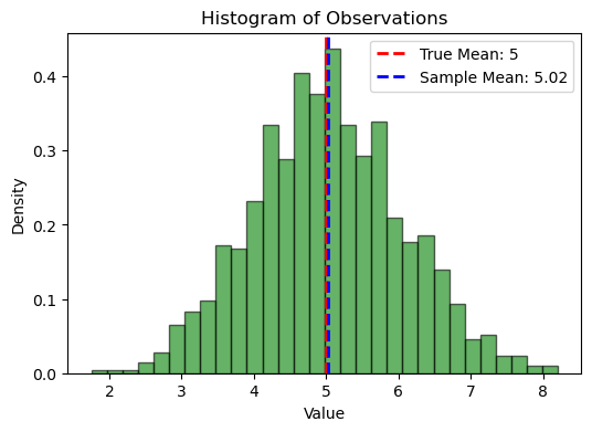
True mean (mu): 5
Sample mean (estimate of mu): 5.020818707346941

Example: Sample Mean and Sample Variance#
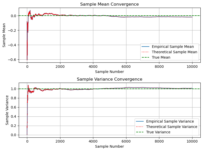
In this example, based on [B2, Ex 10.2], consider the same \( m \) statistically independent Gaussian random variables \( \{ \mathbf{y}_1, \ldots, \mathbf{y}_m \} \) as in previous example.
In a running sum, the sample mean is defined for the current sample \(i\) as
the sample variance is defined for the current sample \(i\) as
# Parameters
m = 10000  # Number of samples
mu = 0  # Mean of the Gaussian random variables
sigma = 1  # Standard deviation of the Gaussian random variables

# Generate m samples of a Gaussian random variable with mean mu and variance sigma^2
y = np.random.normal(mu, sigma, m)

# Initialize arrays to store sample means and variances
empirical_sample_means = np.zeros(m)
empirical_sample_variances = np.zeros(m)
theoretical_sample_mean = np.zeros(m)
theoretical_sample_variances = np.zeros(m)

# Calculate sample mean, sample variance, theoretical mean, and theoretical variance for each sample number
for i in range(1, m + 1):
    empirical_sample_means[i - 1] = np.mean(y[:i])
    empirical_sample_variances[i - 1] = np.var(y[:i], ddof=0)

    # Calculate theoretical sample mean (should be mu for all i)
    theoretical_sample_mean[i - 1] = np.sum(y[:i]) / i

    # Calculate theoretical sample variance using the actual mean at each step
    theoretical_sample_variances[i - 1] = np.sum((y[:i] - np.mean(y[:i]))**2) / i

# Plotting the sample mean and variance as a function of the sample number
fig, axs = plt.subplots(2, 1, figsize=(8, 6))

# Plot Sample Mean
axs[0].plot(range(1, m + 1), empirical_sample_means, label='Empirical Sample Mean')
axs[0].plot(range(1, m + 1), theoretical_sample_mean, 'r:', label='Theoretical Sample Mean')
axs[0].axhline(y=mu, color='g', linestyle='--', label='True Mean')
axs[0].set_title('Sample Mean Convergence')
axs[0].set_xlabel('Sample Number')
axs[0].set_ylabel('Sample Mean')
axs[0].legend()
axs[0].grid(True)

# Plot Sample Variance
axs[1].plot(range(1, m + 1), empirical_sample_variances, label='Empirical Sample Variance')
axs[1].plot(range(1, m + 1), theoretical_sample_variances, 'r:', label='Theoretical Sample Variance')
axs[1].axhline(y=sigma**2, color='g', linestyle='--', label='True Variance')
axs[1].set_title('Sample Variance Convergence')
axs[1].set_xlabel('Sample Number')
axs[1].set_ylabel('Sample Variance')
axs[1].legend()
axs[1].grid(True)

plt.tight_layout()
plt.show()

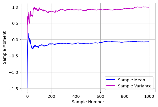
Schonhoff’s Method#
import numpy as np
import matplotlib.pyplot as plt

def zmuv(nsam):
    # Generate samples from a normal distribution with mean=0 and variance=1
    s = np.random.normal(0, 1, nsam)

    # Initialize arrays to store running sums and running variances
    runsum = np.zeros(nsam)
    runm2 = np.zeros(nsam)
    runvar = np.zeros(nsam)

    # Calculate running sums and second moments
    for k in range(nsam):
        runsum[k] = np.sum(s[:k+1]) / (k+1)
        runm2[k] = np.sum(s[:k+1]**2) / (k+1)

    # Calculate running variances
    for j in range(nsam):
        runvar[j] = runm2[j] - runsum[j]**2

    # Plot the results
    plt.figure(figsize=(6, 4))
    plt.plot(runsum, 'b', label='Sample Mean')
    plt.plot(runvar, 'm', label='Sample Variance')
    plt.grid(True)
    plt.ylabel('Sample Moment')
    plt.xlabel('Sample Number')
    plt.legend()
    plt.show()

# Example usage
zmuv(1000)

