Real Scalar Gaussian Random Variable#
Probability Density Function (PDF)#
The probability density function (PDF) of a real scalar Gaussian (normal) random variable \( \mathbf{x} \) with mean \( \mu \) and variance \( \sigma^2 \) is given by:
where:
Mean ( \( \mu \) ): The central value around which the random variable \( \mathbf{x} \) is distributed.
Variance ( \( \sigma^2 \) ): The measure of the spread or dispersion of the random variable around the mean. The standard deviation \( \sigma \) is the square root of the variance.
Exponent Term: The term \( \exp\left(-\frac{(x-\mu)^2}{2\sigma^2}\right) \) describes the bell-shaped curve of the Gaussian distribution. The value decreases exponentially as \( (x-\mu)^2 \) increases, indicating that values further from the mean are less probable.
Normalization Factor: \( \frac{1}{\sqrt{2\pi}\sigma} \) ensures that the total area under the PDF equals 1, a requirement for any probability distribution.
Notation
The notation \( \mathbf{x} \sim \mathcal{N}(\mu, \sigma^2) \) indicates that the random variable \( \mathbf{x} \) follows a Gaussian distribution with mean \( \mu \) and variance \( \sigma^2 \).
Similarly, \( \mathbf{w} \sim \mathcal{N}(0, 1) \) denotes a standard Gaussian (or normal) random variable with mean 0 and variance 1.
Complementary Cumulative Distribution Function (CCDF)#
The complementary cumulative distribution function (CCDF) of the standard Gaussian distribution, denoted as \( Q(a) \), represents the probability that the standard Gaussian random variable \( \mathbf{w} \) exceeds the value \( a \). It is defined as:
This function \( Q(a) \) is often referred to as the Q-function.
It is derived from the tail probability of the standard Gaussian distribution, which is the integral of the probability density function (PDF) from \( a \) to infinity.
DISCUSSION. Behavior of \( Q(a) \) as \( a \) Increases:
When \( a \) is small (close to 0), \( Q(a) \) is relatively large because the probability that \( \mathbf{w} \) exceeds a small number is not negligible.
As \( a \) increases, the area under the curve (from \( a \) to infinity) gets smaller, and so \( Q(a) \) decreases.
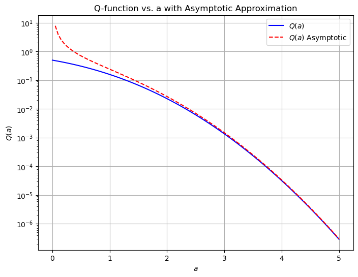
The rate at which \( Q(a) \) decreases as \( a \) increases is very rapid. Specifically, for large values of \( a \), the Q-function behaves approximately as:
\[ Q(a) \approx \frac{1}{a\sqrt{2\pi}} \exp\left(-\frac{a^2}{2}\right) \]This expression shows that \( Q(a) \) decreases much faster than a simple exponential function as \( a \) increases. The leading factor \( \frac{1}{a\sqrt{2\pi}} \) is relatively small compared to the rapid decay caused by the exponential term \( \exp\left(-\frac{a^2}{2}\right) \).
Gaussian decay. When people say “decreases exponentially,” they often refer to functions that decrease like \( e^{-ka} \) for some constant \( k > 0 \). However, \( Q(a) \) decreases even faster because it has a \( -a^2 \) in the exponent. This is known as “Gaussian decay,” which is faster than exponential decay.
import warnings
warnings.filterwarnings("ignore")
import numpy as np
import matplotlib.pyplot as plt
from scipy.special import erfc

# Define the Q-function using the complementary error function
def Q_function(a):
    return 0.5 * erfc(a / np.sqrt(2))

# Generate a range of "a" values
a_values = np.linspace(0, 5, 100)

# Compute the Q-function for each "a"
Q_values = Q_function(a_values)

# Define the asymptotic approximation of the Q-function for large "a"
def Q_function_asymptotic(a):
    return 1 / (a * np.sqrt(2 * np.pi)) * np.exp(-a**2 / 2)

# Compute the asymptotic approximation for each "a"
Q_asymptotic_values = Q_function_asymptotic(a_values)

# Plot both the Q-function and its asymptotic approximation
plt.figure(figsize=(8, 6))
plt.plot(a_values, Q_values, label=r'$Q(a)$', color='blue')
plt.plot(a_values, Q_asymptotic_values, '--', label=r'$Q(a)$ Asymptotic', color='red')
plt.yscale('log')  # Logarithmic scale to emphasize the rapid decrease
plt.xlabel(r'$a$')
plt.ylabel(r'$Q(a)$')
plt.title('Q-function vs. a with Asymptotic Approximation')
plt.grid(True)
plt.legend()
plt.show()

Bounds for \( Q(a) \)#
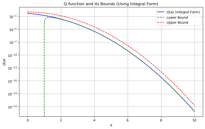
For large values of \( a \), the function \( Q(a) \) can be approximated by the following inequalities:
Lower Bound: The term \( \frac{1}{\sqrt{2\pi}a}\left(1 - \frac{1}{a^2}\right)e^{-\frac{a^2}{2}} \) provides a more precise estimate for large \( a \). It accounts for the \( a^{-1} \) and \( a^{-3} \) terms, refining the exponential decay.
Upper Bound: The simpler bound \( e^{-\frac{a^2}{2}} \) offers a straightforward exponential approximation.
These bounds are useful for estimating probabilities and simplifying calculations involving the tail of the Gaussian distribution, particularly in high-precision contexts such as error rate calculations in communication systems.
Theoretical CDF in Terms of Error Function#
The CDF of a Gaussian (normal) random variable \( \mathbf{x} \sim \mathcal{N}(\mu, \sigma^2) \) can be expressed using the error function (erf).
The error function is defined as:
The CDF of a Gaussian random variable \( \mathbf{x} \) is given by:
For a Gaussian random variable with mean \( \mu \) and variance \( \sigma^2 \), the CDF can be expressed as:
Insights:
Normalization: The argument of the error function \( \frac{x - \mu}{\sigma \sqrt{2}} \) standardizes the variable \( x \) to have a mean of 0 and a variance of 1, aligning it with the standard normal distribution.
Scaling: The factor \( \frac{1}{2} \) scales the range of the error function from \([-1, 1]\) to \([0, 1]\), matching the range of the CDF.
Translation: The \( +1 \) inside the parentheses shifts the result to fit the \([0, 1]\) interval required for the CDF.
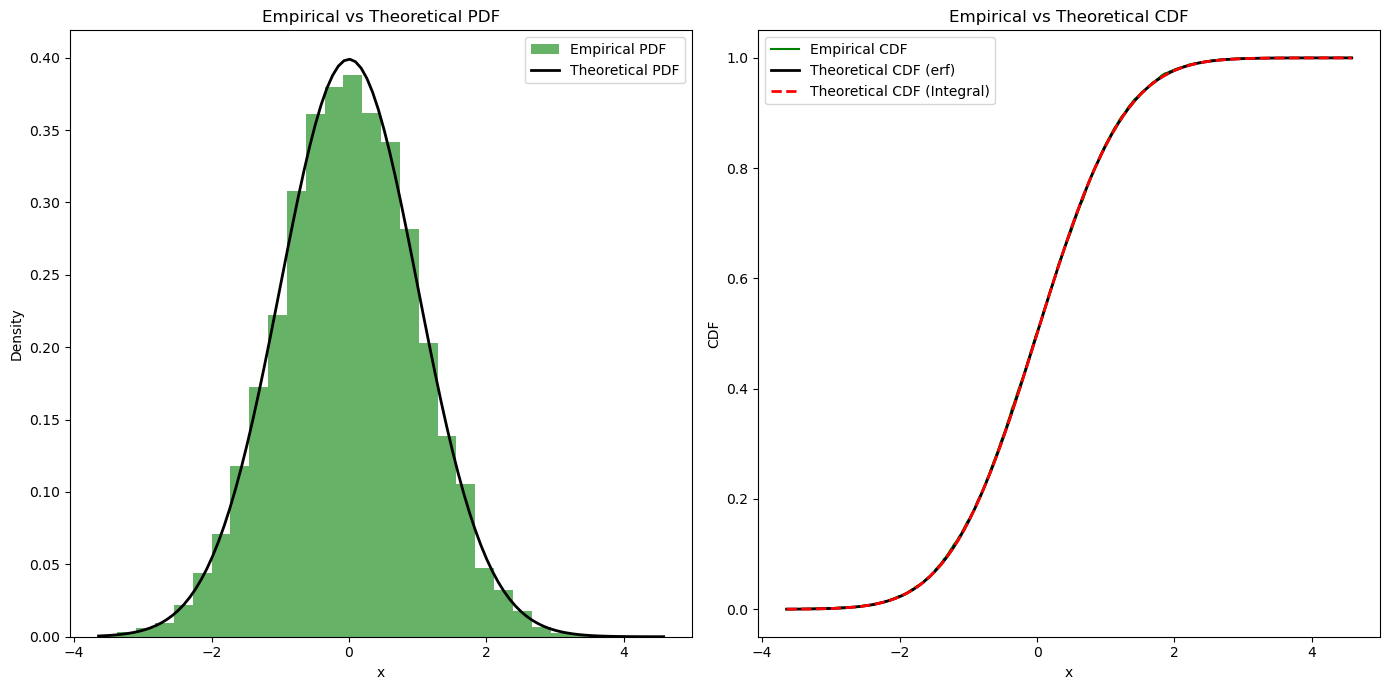
Simulation: Empirical CDF and PDF#
import numpy as np
import matplotlib.pyplot as plt
from scipy.special import erf
from scipy.integrate import quad
import warnings
warnings.filterwarnings("ignore")

# Parameters for the Gaussian distribution
mu = 0       # Mean
sigma = 1    # Standard deviation
num_samples = 10000  # Number of samples

# Step 1: Simulate the real scalar Gaussian random variable
samples = np.random.normal(mu, sigma, num_samples)

# Function to compute the theoretical PDF
def gaussian_pdf(x, mu, sigma):
    return (1 / (np.sqrt(2 * np.pi) * sigma)) * np.exp(-0.5 * ((x - mu) / sigma) ** 2)

# Function to compute the theoretical CDF using the error function
def gaussian_cdf_erf(x, mu, sigma):
    return 0.5 * (1 + erf((x - mu) / (sigma * np.sqrt(2))))

# Function to compute the theoretical CDF using the Q-function integral
def gaussian_cdf_integral(x, mu, sigma):
    Q_a = lambda a: (1 / np.sqrt(2 * np.pi)) * np.exp(-0.5 * a ** 2)
    cdf_values = []
    for value in x:
        integral, _ = quad(Q_a, value, np.inf)
        cdf_value = 1 - integral
        cdf_values.append(cdf_value)
    return np.array(cdf_values)

# Step 2: Plot the empirical PDF
plt.figure(figsize=(14, 7))

# Histogram for empirical PDF
plt.subplot(1, 2, 1)
count, bins, ignored = plt.hist(samples, bins=30, density=True, alpha=0.6, color='g', label='Empirical PDF')

# Plot the theoretical PDF
x = np.linspace(min(bins), max(bins), 100)
pdf = gaussian_pdf(x, mu, sigma)
plt.plot(x, pdf, 'k', linewidth=2, label='Theoretical PDF')
plt.title('Empirical vs Theoretical PDF')
plt.xlabel('x')
plt.ylabel('Density')
plt.legend()

# Step 3: Plot the theoretical CDF and compare with the empirical CDF
# Empirical CDF
empirical_cdf = np.arange(1, num_samples + 1) / num_samples
sorted_samples = np.sort(samples)

plt.subplot(1, 2, 2)
plt.step(sorted_samples, empirical_cdf, label='Empirical CDF', color='g')

# Theoretical CDF using error function
cdf_erf = gaussian_cdf_erf(x, mu, sigma)
plt.plot(x, cdf_erf, 'k', linewidth=2, label='Theoretical CDF (erf)')

# Theoretical CDF using the integral of Q-function
cdf_integral = gaussian_cdf_integral(x, mu, sigma)
plt.plot(x, cdf_integral, 'r--', linewidth=2, label='Theoretical CDF (Integral)')

plt.title('Empirical vs Theoretical CDF')
plt.xlabel('x')
plt.ylabel('CDF')
plt.legend()

plt.tight_layout()
plt.show()

Discussions on the bounds#
The bounds of \( Q(a) \), the complementary CDF of the standard Gaussian distribution, are derived using asymptotic approximations and properties of the Gaussian distribution.
The complementary CDF \( Q(a) \) is defined as:
Asymptotic Approximation for Large \( a \)
For large values of \( a \), the value of \( Q(a) \) can be approximated by examining the behavior of the integrand \( \exp\left(-\frac{w^2}{2}\right) \). The idea is to find simpler expressions that approximate the integral accurately.
Using the Tail Probability Approximation
For large \( a \), the value of the integral \( Q(a) \) is dominated by the values of \( \mathbf{w} \) close to \( a \). Therefore, we can approximate the tail probability by considering the leading terms of the integrand’s expansion.
Applying the Change of Variable Technique
One common approach is to perform a change of variables to simplify the integration. Let’s use the complementary error function, denoted as \( \text{erfc}(a) \), which is related to \( Q(a) \):
The complementary error function for large \( a \) can be approximated using the asymptotic expansion:
For \( z = \frac{a}{\sqrt{2}} \), we have:
Therefore, \( Q(a) \) can be approximated as:
Lower Bound Derivation
The lower bound is derived from the above approximation. For large \( a \), we can drop higher-order terms and keep the leading terms:
Thus, the lower bound for \( Q(a) \) is:
Upper Bound Derivation
The upper bound can be found by recognizing that \( Q(a) \) is always less than the simple exponential term because the integrand \( \exp\left(-\frac{w^2}{2}\right) \) decreases rapidly:
For large \( a \), the upper bound is dominated by the leading exponential term without the need for additional terms:
Combining these results, we get the bounds for \( Q(a) \) for large \( a \):
These bounds are very useful in practice because they provide a simple yet accurate way to estimate the tail probabilities of the Gaussian distribution, which is particularly important in statistical analysis and communication theory.
import numpy as np
import matplotlib.pyplot as plt
from scipy.integrate import quad

# Define the Q-function using the integral form
def Q_function_integral(a):
    integrand = lambda w: (1 / np.sqrt(2 * np.pi)) * np.exp(-w**2 / 2)
    result, _ = quad(integrand, a, np.inf)
    return result

# Define the lower bound of Q(a)
def lower_bound_Q(a):
    return (1 / (np.sqrt(2 * np.pi) * a)) * (1 - 1 / a**2) * np.exp(-a**2 / 2)

# Define the upper bound of Q(a)
def upper_bound_Q(a):
    return np.exp(-a**2 / 2)

# Values of a to evaluate
a_values = np.linspace(0, 10, 500)

# Compute Q(a) and its bounds
Q_values = np.array([Q_function_integral(a) for a in a_values])
lower_bounds = lower_bound_Q(a_values)
upper_bounds = upper_bound_Q(a_values)

# Plot Q(a) and its bounds
plt.figure(figsize=(10, 6))
plt.plot(a_values, Q_values, label='$Q(a)$ (Integral Form)', color='blue')
plt.plot(a_values, lower_bounds, '--', label='Lower Bound', color='green')
plt.plot(a_values, upper_bounds, '--', label='Upper Bound', color='red')
plt.xlabel('$a$')
plt.ylabel('$Q(a)$')
plt.yscale('log')
plt.title('Q-function and its Bounds (Using Integral Form)')
plt.legend()
plt.grid(True)
plt.show()

