Central Limit Theorem#
The Central Limit Theorem (CLT) is a fundamental result in probability and statistics that applies to situations where we observe an experiment repeatedly under the assumption of independent and identical random phenomena. This theorem explains how the behavior of the sample mean of random variables converges to a normal distribution under certain conditions.
Independent and Identically Distributed (IID) Random Variables#
Definition
A sequence of random variables \( X_1, X_2, \ldots, X_n \) is said to be independent and identically distributed (IID) if the following conditions are satisfied:
Identically Distributed:
Each random variable \( X_i \) has the same cumulative distribution function (CDF), \( F_{X_i}(x) = F_X(x) \), for all \( i = 1, 2, \ldots, n \).This means that every \( X_i \) follows the same probability distribution.
Independence:
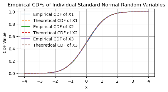
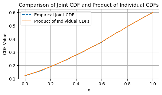
The joint CDF of the random variables is the product of their individual CDFs:\[ F_{X_1, X_2, \ldots, X_n}(x_1, x_2, \ldots, x_n) = \prod_{i=1}^{n} F_{X_i}(x_i). \]This implies that the variables do not influence one another, and the outcome of one variable has no effect on the others.
Practical Significance
Repeated Observations: In many real-world scenarios, we observe multiple outcomes of an experiment or process, each corresponding to an independent realization of the underlying random phenomenon.
CLT Application: The IID assumption is crucial for the Central Limit Theorem, as it ensures that the sample mean behaves predictably, converging to a normal distribution as the number of observations increases.
import numpy as np
import matplotlib.pyplot as plt
from scipy.stats import norm


# Define the parameters
n = 3  # Number of random variables
num_samples = 10000  # Number of samples to simulate
x_values = np.linspace(0, 1, 100)  # Values for the CDF

# Generate n independent random variables from a standard normal distribution (mean=0, std=1)
random_vars_standard_normal = [np.random.normal(0, 1, num_samples) for _ in range(n)]

# Define a wider range of x values to cover the tails of the standard normal distribution
x_values_standard_normal = np.linspace(-4, 4, 200)

# Plot the individual CDFs of each standard normal random variable
plt.figure(figsize=(6, 3))

for i, var in enumerate(random_vars_standard_normal):
    empirical_cdf = [np.mean(var <= x) for x in x_values_standard_normal]
    plt.plot(x_values_standard_normal, empirical_cdf, label=f'Empirical CDF of X{i+1}')

    theoretical_cdf = norm.cdf(x_values_standard_normal)
    plt.plot(x_values_standard_normal, theoretical_cdf, label=f'Theoretical CDF of X{i+1}', linestyle='--')


plt.xlabel('x')
plt.ylabel('CDF Value')
plt.title('Empirical CDFs of Individual Standard Normal Random Variables')
plt.legend()
plt.grid()
plt.show()


# Calculate the empirical joint CDF
joint_cdf_values = []
for x in x_values:
    joint_cdf_values.append(np.mean(np.all([var <= x for var in random_vars_standard_normal], axis=0)))

# Calculate the product of individual CDFs
individual_cdfs = [np.mean(var <= x_values[:, None], axis=1) for var in random_vars_standard_normal]
product_cdf_values = np.prod(individual_cdfs, axis=0)

# Plot the results
plt.figure(figsize=(6, 3))
plt.plot(x_values, joint_cdf_values, label='Empirical Joint CDF', linestyle='--')
plt.plot(x_values, product_cdf_values, label='Product of Individual CDFs', linestyle='-')
plt.xlabel('x')
plt.ylabel('CDF Value')
plt.title('Comparison of Joint CDF and Product of Individual CDFs')
plt.legend()
plt.grid()
plt.show()
Limit Theorems for Sums of Random Variables#
When dealing with a sequence of independent and identically distributed (IID) random variables \( \{X_i, i = 1, 2, 3, \ldots \} \), it is intuitive to expect that the sample mean, also known as, running average:
should converge, in some sense, to the expected value (mean) of the random variables as the number of observations \( n \) becomes large.
The Limit Theorems#
Two fundamental theorems provide a rigorous framework for understanding how the running average \( Y_n \) behaves as \( n \to \infty \):
Law of Large Numbers (LLN):
The LLN states that, as \( n \) grows, the sample mean \( Y_n \) converges to the true mean \( \mathbb{E}[X] \) of the random variable \( X \).
This convergence can be interpreted in different senses (e.g., almost surely or in probability), depending on the version of the LLN being considered (Strong LLN or Weak LLN).
Central Limit Theorem (CLT):
The CLT provides a deeper insight into the distribution of the sample mean \( Y_n \). It states that, for sufficiently large \( n \), the distribution of the scaled deviation:
\[ \sqrt{n} \left(Y_n - \mathbb{E}[X]\right) \]approaches a normal distribution with mean 0 and variance equal to the variance of \( X \), \( \sigma^2 = \text{Var}(X) \).
This result explains why the normal distribution arises so frequently in statistics and nature.
Key Intuitions
LLN: Guarantees that \( Y_n \) gets closer to the true mean \( \mathbb{E}[X] \) as \( n \) increases.
CLT: Describes the variability of \( Y_n \) around \( \mathbb{E}[X] \) for large \( n \), showing that the fluctuations follow a normal distribution.
Practical Significance
These limit theorems form the cornerstone of statistical inference, underpinning the validity of approximations, confidence intervals, and hypothesis testing.
The LLN ensures the reliability of long-term averages, while the CLT provides tools for quantifying uncertainty in estimates.
The Law of Large Numbers (LLN)#
The law of large numbers (LLN) is a foundational result in probability theory that formalizes the intuitive idea that the sample mean of a sequence of random variables converges to their expected value as the sample size becomes very large.
Theorem: Strong Law of Large Numbers (S-LLN)#
Let \( \{X_i, i = 1, 2, \ldots\} \) be a sequence of independent and identically distributed (IID) random variables with finite mean \( \mathbb{E}[X_1] < \infty \).
Then, the S-LLN is stated as [Proakis, Eq. (2.5-2)]:
as \( n \to \infty \).
Type of Convergence
The convergence described by the strong law of large numbers is almost everywhere (a.e.) or almost surely (a.s.). This means that:
For almost every outcome in the probability space, the sample mean converges to the expected value.
The probability of the set of outcomes where convergence does not occur is zero.
In mathematical terms:
For a sequence of independent and identically distributed (IID) random variables \( \{X_1, X_2, \ldots, X_n\} \), the following holds:
Identical Expected Value
where \( \mu \) is the true mean of the underlying distribution. Since all the random variables share the same distribution, they also share the same expected value.
The equality \( \mathbb{E}[X_1] = \mathbb{E}[X_2] = \cdots = \mathbb{E}[X_n] \) ensures that the sequence of random variables behaves consistently in expectation, which is a key requirement for applying the SLLN.
True Mean
The term “true mean” refers to this common expected value \( \mu \). It represents the theoretical average value of the random variable if we could sample infinitely many observations.
Sample Mean Convergence
The Strong Law of Large Numbers (SLLN) states that the sample mean:
converges to \( \mu \) (the true mean) as \( n \to \infty \). This means that with a large enough sample size, the sample mean becomes a reliable estimator of the true mean.
The formal way to express the Strong Law of Large Numbers is:
where:
\( \xrightarrow{\text{a.s.}} \): This symbol denotes almost sure convergence, which means that the sequence of random variables \( \frac{1}{n} \sum_{i=1}^n X_i \) converges to \( \mu \) with probability 1 as \( n \to \infty \).
Practical Implications
The LLN ensures that repeated sampling or experimentation yields results that approach the true mean of the population.
It justifies why averages of large samples are reliable estimates of the population mean in fields such as economics, physics, and data science.
Example: S-LLN for Standard Normal RV#
For a standard normal distribution (\( N(0, 1) \)):
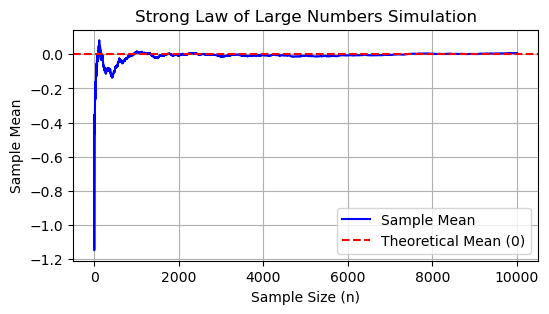
\( \mathbb{E}[X_1] = \mathbb{E}[X_2] = \cdots = \mathbb{E}[X_n] = 0 \), so \( \mu = 0 \), the true mean.
This property guarantees that the sample mean calculated from the sequence will converge to 0 as \( n \to \infty \).
# Parameters
num_iterations = 10000  # Total number of random variables (sequence size)
sample_sizes = range(1, num_iterations + 1)  # Incremental sample sizes

# Define X1 as the first random variable from a standard normal distribution
X1 = np.random.normal(0, 1)

# Generate the rest of the sequence X2, X3, ..., Xn
rest_of_sequence = np.random.normal(0, 1, num_iterations - 1)

# Combine X1 and the rest of the sequence to form the full sequence
full_sequence = np.concatenate(([X1], rest_of_sequence))

# Compute cumulative sample means
sample_means = [np.mean(full_sequence[:n]) for n in sample_sizes]

# Theoretical mean of a standard normal distribution
theoretical_mean = 0

# Plot the convergence of the sample mean
plt.figure(figsize=(6, 3))
plt.plot(sample_sizes, sample_means, label='Sample Mean', linestyle='-', color='blue')
plt.axhline(theoretical_mean, color='red', linestyle='--', label='Theoretical Mean (0)')
plt.xlabel('Sample Size (n)')
plt.ylabel('Sample Mean')
plt.title('Strong Law of Large Numbers Simulation')
plt.legend()
plt.grid()
plt.show()
The Central Limit Theorem (CLT)#
The central limit theorem (CLT) is a cornerstone of probability and statistics. It explains how the distribution of the sample mean of a sequence of random variables converges to a normal distribution, regardless of the original distribution of the variables, provided certain conditions are met.
Theorem: Central Limit Theorem#
Let \( \{X_i, i = 1, 2, \ldots\} \) be a sequence of independent and identically distributed (IID) random variables with:
True mean: \( \mu = \mathbb{E}[X_1] < \infty \),
Variance: \( \sigma^2 = \text{Var}[X_1] < \infty \).
Then, the standardized sum of these variables:
converges in distribution to a standard normal random variable:
as \( n \to \infty \).
Implications
Standardization:
The numerator \( \frac{1}{n} \sum_{i=1}^n X_i - \mu \) represents the deviation of the sample mean from the true mean.
The denominator \( \frac{\sigma}{\sqrt{n}} \) scales this deviation by the standard error, accounting for variability and sample size.
Type of Convergence:
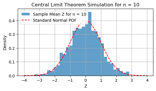
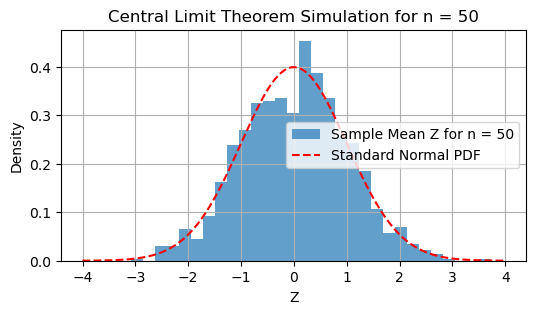
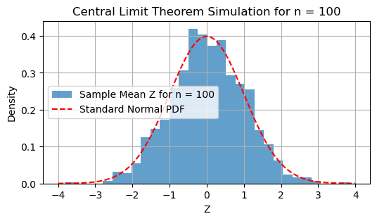
The convergence described in the CLT is convergence in distribution, which means that the cumulative distribution function (CDF) of \( Z \) approaches the CDF of a standard normal distribution \( \mathcal{N}(0, 1) \) as \( n \) becomes large.
Practical Implications
Normal Approximation:
For sufficiently large \( n \), the distribution of the sample mean can be approximated by a normal distribution, even if the original \( X_i \) are not normally distributed.
Foundation for Statistical Inference:
The CLT justifies the use of normal distribution-based methods for hypothesis testing, confidence intervals, and other inferential techniques.
# Parameters for the simulation
import numpy as np
import matplotlib.pyplot as plt
import scipy.stats as stats

num_trials = 1000  # Number of trials for approximating the distribution of Z
n_values = [10, 50, 100, 50000]  # Different sample sizes to show convergence

# True mean and variance of the distribution
mu = 13  # Mean of the distribution
sigma = 13  # Standard deviation of the distribution

# Simulation to compute Z for different sample sizes
for n in n_values:

    # Simulate num_trials sets of size n to approximate Z
    trials = np.random.normal(mu, sigma, (num_trials, n))
    trial_means = np.mean(trials, axis=1)

    # Standardize the sample means to compute Z
    Z_values = (trial_means - mu) / (sigma / np.sqrt(n))

    # Plot the histogram of Z values
    plt.figure(figsize=(6, 3))
    plt.hist(Z_values, bins=30, density=True, alpha=0.7, label=f'Sample Mean Z for n = {n}')

    # Overlay the theoretical standard normal distribution
    x = np.linspace(-4, 4, 500)
    plt.plot(x, stats.norm.pdf(x, 0, 1), label='Standard Normal PDF', color='red', linestyle='--')

    plt.title(f'Central Limit Theorem Simulation for n = {n}')
    plt.xlabel('Z')
    plt.ylabel('Density')
    plt.legend()
    plt.grid()
    plt.show()

Applied to the Gamma Distribution#
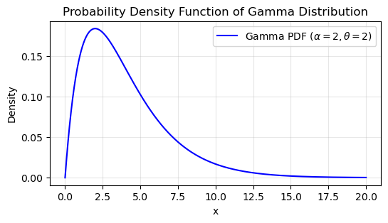
The probability density function (PDF) of the Gamma distribution is given by:
where:
\( \alpha \) (shape parameter) determines the shape of the distribution.
\( \theta \) (scale parameter) stretches or compresses the distribution horizontally.
\( \Gamma(\alpha) \) is the Gamma function, defined as:
\[ \Gamma(\alpha) = \int_0^\infty t^{\alpha - 1} e^{-t} \, dt. \]
The Gamma distribution, parameterized by the shape parameter \( k \) (or \( \alpha \)) and scale parameter \( \theta \), has the following properties:
Mean:
\[ \mu = k \cdot \theta \]Variance:
\[ \sigma^2 = k \cdot \theta^2 \]
Let \( X_1, X_2, \ldots, X_n \) be independent and identically distributed (IID) random variables from a Gamma distribution, such that \( X_i \sim \text{Gamma}(k, \theta) \). The sample mean is defined as:
To standardize this sample mean, we use:
where \( \mu = k \cdot \theta \) is the true mean, and \( \sigma = \sqrt{k \cdot \theta^2} \) is the standard deviation. Substituting these values, \( Z_n \) becomes:
Convergence to the Standard Normal Distribution
As \( n \to \infty \), the distribution of \( Z_n \) converges in distribution to the standard normal distribution:
This implies:
The sample mean \( \bar{X}_n \) remains centered around the true mean \( \mu = k \cdot \theta \).
The variability of \( \bar{X}_n \), scaled by \( \sqrt{n} \), decreases, leading to a closer approximation of the standard normal distribution.
Verification via Simulation#
The histogram simulation verifies the Central Limit Theorem (CLT). As \( n \) increases, the distribution of the standardized sample means (\( Z_n \)) increasingly resembles the standard normal distribution. This is a direct consequence of the CLT, as the effects of the Gamma distribution’s shape diminish with larger sample sizes.
import numpy as np
import matplotlib.pyplot as plt
import scipy.stats as stats

# Parameters for the Gamma distribution
shape_param = 2  # Shape parameter (alpha)
scale_param = 2  # Scale parameter (theta)

# Generate x values for plotting
x = np.linspace(0, 20, 1000)  # Range of x values

# Compute the PDF of the Gamma distribution
pdf = stats.gamma.pdf(x, a=shape_param, scale=scale_param)

# Plot the PDF
plt.figure(figsize=(6, 3))
plt.plot(x, pdf, label=f"Gamma PDF ($\\alpha={shape_param}, \\theta={scale_param}$)", color='blue')
plt.title("Probability Density Function of Gamma Distribution")
plt.xlabel("x")
plt.ylabel("Density")
plt.grid(alpha=0.3)
plt.legend()
plt.show()


# Simulation parameters
n_samples = 1000  # Number of samples per simulation
sample_sizes = [1, 5, 10, 30, 50, 100]  # Varying sample sizes for the CLT demonstration
n_simulations = 10000  # Number of simulations

# True mean and variance of the Gamma distribution
true_mean = shape_param * scale_param
true_variance = shape_param * scale_param**2
true_std = np.sqrt(true_variance)

# Collecting standardized means for each sample size
standardized_means = {}

for n in sample_sizes:
    sample_means = []
    for _ in range(n_simulations):
        sample = np.random.gamma(shape_param, scale_param, n)
        sample_mean = np.mean(sample)
        standardized_mean = (sample_mean - true_mean) / (true_std / np.sqrt(n))
        sample_means.append(standardized_mean)
    standardized_means[n] = sample_means

# Plotting the results
plt.figure(figsize=(15, 5))
for i, n in enumerate(sample_sizes, 1):
    plt.subplot(2, 3, i)
    plt.hist(standardized_means[n], bins=50, density=True, alpha=0.6, label=f'Sample size = {n}')

    # Plot standard normal PDF for reference
    x = np.linspace(-4, 4, 500)
    plt.plot(x, stats.norm.pdf(x), 'r-', lw=2, label='Standard Normal PDF')

    plt.title(f'Standardized Means (n = {n})')
    plt.xlabel('Z')
    plt.ylabel('Density')
    plt.legend()

plt.tight_layout()
plt.show()

Applied to the Poisson Distribution#
Definition of the Poisson Random Variable (RV)#
A Poisson random variable \( X \) represents the number of events occurring in a fixed interval of time or space, assuming:
Events occur independently.
The average rate (\( \lambda \)) of events is constant.
The probability of more than one event occurring in an infinitesimally small interval is negligible.
The Poisson random variable is parameterized by:
\( \lambda > 0 \): the rate (or mean) of occurrences in the interval.
Probability Mass Function (PMF)#
The PMF of a Poisson RV is defined as:
where:
\( k \): the number of events (a non-negative integer).
\( \lambda \): the mean and variance of the Poisson distribution.
True Mean#
For a Poisson random variable \( X \sim \text{Poisson}(\lambda) \), the mean is:
True Variance#
The variance of a Poisson RV is equal to its mean:
Standardized Sample Mean (Z)#
Given \( n \) independent and identically distributed (IID) Poisson random variables \( X_1, X_2, \ldots, X_n \), the sample mean is:
To standardize \( \bar{X}_n \), we use the formula:
Substituting \( \mu = \lambda \) and \( \sigma = \sqrt{\lambda} \):
Central Limit Theorem (CLT)#
As the sample size \( n \to \infty \), the distribution of the standardized sample mean \( Z_n \) converges to the standard normal distribution:
This means:
The mean of \( Z_n \) approaches 0.
The variance of \( Z_n \) approaches 1.
Visualization in the Code#
CLT Demonstration:
The simulation generates multiple samples from a Poisson distribution with \( \lambda = 5 \) for varying sample sizes (\( n \)).
It calculates the standardized sample mean (\( Z_n \)) and plots histograms to show the convergence to the standard normal distribution as \( n \) increases.
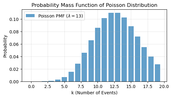
PMF of a Single Poisson RV:
The code calculates the PMF values for \( k = 0, 1, 2, \ldots, 19 \) using the formula above and plots it to visualize the probability distribution of a Poisson RV with \( \lambda = 5 \).
import numpy as np
import warnings
import matplotlib.pyplot as plt
import scipy.stats as stats

warnings.filterwarnings('ignore')

# Parameters for the Poisson distribution
lambda_param = 13  # Rate parameter (mean of the Poisson distribution)

# Simulation parameters
sample_sizes = [1, 5, 10, 30, 50, 100]  # Varying sample sizes for the CLT demonstration
n_simulations = 10000  # Number of simulations

# True mean and variance of the Poisson distribution
true_mean = lambda_param
true_variance = lambda_param
true_std = np.sqrt(true_variance)

# Collecting standardized means for each sample size
standardized_means_poisson = {}

for n in sample_sizes:
    sample_means = []
    for _ in range(n_simulations):
        sample = np.random.poisson(lambda_param, n)
        sample_mean = np.mean(sample)
        standardized_mean = (sample_mean - true_mean) / (true_std / np.sqrt(n))
        sample_means.append(standardized_mean)
    standardized_means_poisson[n] = sample_means

# Plotting the PDF of a single Poisson RV
k = np.arange(0, 20, 1)  # Values for which the PMF will be calculated
poisson_pmf = stats.poisson.pmf(k, mu=lambda_param)

plt.figure(figsize=(6, 3))
plt.bar(k, poisson_pmf, alpha=0.7, label=f'Poisson PMF ($\lambda={lambda_param}$)')
plt.title("Probability Mass Function of Poisson Distribution")
plt.xlabel("k (Number of Events)")
plt.ylabel("Probability")
plt.grid(alpha=0.3)
plt.legend()
plt.show()

# Plotting the results
plt.figure(figsize=(15, 5))
for i, n in enumerate(sample_sizes, 1):
    plt.subplot(2, 3, i)
    plt.hist(standardized_means_poisson[n], bins=50, density=True, alpha=0.6, label=f'Sample size = {n}')

    # Plot standard normal PDF for reference
    x = np.linspace(-4, 4, 500)
    plt.plot(x, stats.norm.pdf(x), 'r-', lw=2, label='Standard Normal PDF')

    plt.title(f'Standardized Means (n = {n})')
    plt.xlabel('Z')
    plt.ylabel('Density')
    plt.legend()

plt.tight_layout()
plt.show()
