Whitening with Eigenvalue Decomposition (EVD)#
Example of the whitening process, assuming the transmitted signal \( s_m \) is a 4-QAM signal, and the whitening matrix \( W \) is computed via eigenvalue decomposition (EVD).
Signal Modelling#
Suppose we have the received vector (for simplicity, assume length \(N\)):
\( s_m \) is a symbol from a 4-QAM constellation, such as:
\( \vec{n} \) is a colored noise vector with covariance:
Compute Noise Covariance Matrix \( R_n \)#
In practice, the covariance matrix \( R_n \) of the noise is known or estimated:
Typically, this matrix is Hermitian (i.e., \(R_n = R_n^H\)), and positive definite.
Eigenvalue Decomposition of \( R_n \)#
Perform Eigenvalue Decomposition (EVD) of \( R_n \):
\( U \) is a unitary matrix whose columns are the eigenvectors of \( R_n \).
\( \Lambda \) is a diagonal matrix containing positive eigenvalues of \( R_n \):
These eigenvalues represent the noise power distribution across directions.
Construct the Whitening Matrix \( W \)#
The whitening filter \( W \) is constructed as:
where:
\( \Lambda^{-1/2} \) is a diagonal matrix obtained by taking the inverse square root of each eigenvalue:
Thus:
This transformation aligns the noise eigenvectors and normalizes the variance to unity, removing correlations.
Apply Whitening Matrix to Received Signal#
Transform the received signal \(\vec{r}\) using the whitening matrix \(W\):
Define:
\( W s_m \): Transformed signal (still from 4-QAM, but rotated/scaled).
\( W \vec{n} = \vec{v} \): White noise vector (now has identity covariance \( I \)).
Thus, we have:
After whitening, the noise is uncorrelated with identical variance (white noise).
Perform Detection on the Whitened Signal#
Since \(\vec{\rho}\) now has white noise, optimal detection simplifies to comparing against transformed 4-QAM constellation points:
Compute reference points \( W s_m \) for each possible transmitted 4-QAM symbol.
Apply a standard Euclidean-distance-based detector:
This step is now straightforward due to the whitened noise structure.
Recover Original Signal#
If the goal includes reconstructing the original received vector from the whitened vector, simply apply the inverse of \( W \):
Since \(W\) is invertible, no information loss occurs.
Simulation#
Set the noise covariance matrix \(R_n\).
Eigen-decompose \(R_n = U\Lambda U^H\).
Construct \(W = \Lambda^{-1/2}U^H\).
Whiten received vector: \(\vec{\rho}= W \vec{r}\).
Detect the symbol from whitened vector \(\vec{\rho}\).
Simulation Setup#
4-QAM Constellation:
The constellation points are:\[ \{[1, 1], [1, -1], [-1, 1], [-1, -1]\} \]Each point represents 2 bits:
[1, 1] → 00
[1, -1] → 01
[-1, 1] → 10
[-1, -1] → 11
Noise:
The noise vector \(\vec{n}\) has a covariance matrix:\[\begin{split} R_n = \begin{bmatrix} 4 & 2 \\ 2 & 3 \end{bmatrix} \end{split}\]The noise power is scaled to vary the Signal-to-Noise Ratio (SNR).
Detector:
A Nearest Neighbor Detector is used.
Symbols are detected by selecting the constellation point minimizing the Euclidean distance.
Simulation Steps:#
Generate random 4-QAM symbols and colored noise for different SNR values.
Compute received signal:
\[ \vec{r} = s_m + \vec{n} \]Apply whitening filter:
\[ \vec{\rho} = W \vec{r} \]Perform detection:
Direct detection using \(\vec{r}\) (against the original constellation).
Detection using \(\vec{\rho}\) (against the whitened constellation \(W s_m\)).
Calculate the Bit Error Rate (BER):
Compare detected bits to transmitted bits.
import numpy as np
import matplotlib.pyplot as plt
from scipy.stats import gaussian_kde

# Set random seed for reproducibility
np.random.seed(42)

# Parameters
qam_symbols = np.array([[1, 1], [1, -1], [-1, 1], [-1, -1]])  # 4-QAM [Re, Im]
bit_mapping = {tuple([1, 1]): [0, 0], tuple([1, -1]): [0, 1],
               tuple([-1, 1]): [1, 0], tuple([-1, -1]): [1, 1]}  # Original symbol to bits
inv_bit_mapping = {(0, 0): [1, 1], (0, 1): [1, -1],
                   (1, 0): [-1, 1], (1, 1): [-1, -1]}  # Bits to original symbol
num_bits = 100000  # Total bits
num_symbols = num_bits // 2  # 2 bits per symbol
Eb_N0_dB_range = np.arange(0, 15, 2)  # Eb/N0 range in dB
Eb_N0_dB_for_pdf = 6  # Eb/N0 for PDF comparison
import numpy as np

# Noise covariance
R_n_base = np.array([[4, 2],
                [2, 3]], dtype=float)

# Eigen-decomposition
vals, vecs = np.linalg.eig(R_n_base)

# Sort eigenvalues (descending) and reorder eigenvectors accordingly
idx = np.argsort(vals)[::-1]    # indices that would sort eigenvalues descending
vals = vals[idx]
vecs = vecs[:, idx]

# Construct Lambda^{-1/2}  (inverse sqrt of eigenvalues)
Lambda_inv_sqrt = np.diag(1.0 / np.sqrt(vals))

# W = Lambda^{-1/2} * U^T
W = Lambda_inv_sqrt @ vecs.T
W_inv = np.linalg.inv(W)  # Inverse of W

# Display results
print("\nNumerical Whitening Filter:")
print(W)

# Verify
verification = W @ R_n_base @ W.T
print("\nVerification (W R_n W^T, should be close to I):")
print(verification)
Numerical Whitening Filter:
[[ 0.33422689  0.26095647]
 [-0.51312024  0.6571923 ]]

Verification (W R_n W^T, should be close to I):
[[ 1.00000000e+00 -1.31007558e-16]
 [-1.52948929e-16  1.00000000e+00]]
We manually derive the whitening matrix \( W \) for the given noise covariance matrix:
Compute Eigenvalues of \( R_n \)
The eigenvalues are found by solving:
Expanding the determinant,
Solving the quadratic equation,
Approximating,
Compute Eigenvectors of \( R_n \)
For \( \lambda_1 = \frac{7 + \sqrt{17}}{2} \), solve:
Substituting \( \lambda_1 \approx 5.5616 \):
Setting the first equation \( -1.5616 x + 2y = 0 \) gives:
Choosing \( x = 1 \), we get:
Normalizing:
For \( \lambda_2 = \frac{7 - \sqrt{17}}{2} \), solving similarly, we get:
Form \( \Lambda^{-1/2} \)
Approximating:
Compute Whitening Matrix \( W = \Lambda^{-1/2} U^T \)
Multiplying:
Thus, the exact numeric whitening matrix \( W \) is:
Note.
NumPy’s np.linalg.eigh sorts eigenvalues in ascending order (\(\lambda_1 = 1, \lambda_2 = 3\)), which swaps the columns of \( U \) and the diagonal elements of \(\Lambda\).
This is the standard eigenvector sign ambiguity.
In an eigen‐decomposition, each eigenvector is only determined up to a factor of \(\pm1\). Flipping the sign of one eigenvector column (or row in \(W\)) does not change the fact that it is a valid whitening transform.
Concretely, if \(\mathbf{v}\) is an eigenvector, then so is \(-\mathbf{v}\). In the whitening matrix \(W = \Lambda^{-\tfrac12}U^T\), flipping one column’s sign in \(U\) flips the corresponding row in \(W\). Either choice yields the same whitening effect, because
So the “Numerical” \(W\) and “Theoretical” \(W\) differ only by a sign flip in the second row, but both correctly whiten the covariance.
# Whitened constellation
qam_symbols_whitened = (W @ qam_symbols.T).T

# Energy per bit
Es = np.mean(np.sum(qam_symbols**2, axis=1))  # Symbol energy = 2
Eb = Es / 2  # Energy per bit = 1

# Detection function
def detect_symbols(received, constellation):
    detected = np.zeros(received.shape, dtype=float)
    for i in range(received.shape[1]):
        distances = np.sum((constellation - received[:, i][:, np.newaxis])**2, axis=0)
        detected[:, i] = constellation[:, np.argmin(distances)]
    return detected

# Demodulate symbols to bits
def demodulate_symbols(detected_symbols, constellation, bit_mapping, is_whitened=False, W_inv=None):
    if is_whitened:
        detected_original = W_inv @ detected_symbols
        detected_clean = detect_symbols(detected_original, qam_symbols.T)
    else:
        detected_clean = detect_symbols(detected_symbols, qam_symbols.T)
    return np.array([bit_mapping[tuple(detected_clean[:, i])]
                     for i in range(detected_clean.shape[1])]).flatten()

# Function to plot scatter and PDFs
def plot_comparison(data1, data2, label1, label2, title):
    plt.figure(figsize=(12, 5))

    # Scatter plot
    plt.subplot(1, 2, 1)
    plt.scatter(data1[0, :], data1[1, :], alpha=0.2, label=label1, s=10)
    plt.scatter(data2[0, :], data2[1, :], alpha=0.2, label=label2, s=10)
    plt.xlabel('Real/Component 1')
    plt.ylabel('Imag/Component 2')
    plt.legend()
    plt.title(f'Scatter: {title}')

    # PDFs
    plt.subplot(1, 2, 2)
    for i, comp in enumerate(['Real', 'Imag']):
        kde1 = gaussian_kde(data1[i, :])
        kde2 = gaussian_kde(data2[i, :])
        x = np.linspace(min(data1[i, :].min(), data2[i, :].min()),
                        max(data1[i, :].max(), data2[i, :].max()), 100)
        plt.plot(x, kde1(x), label=f'{label1} {comp}')
        plt.plot(x, kde2(x), label=f'{label2} {comp}')
    plt.xlabel('Value')
    plt.ylabel('Density')
    plt.legend()
    plt.title(f'PDFs: {title}')

    plt.tight_layout()
    plt.show()
# Generate binary sequence and map to 4-QAM
bits_tx = np.random.randint(0, 2, num_bits)
s_m_samples = np.array([inv_bit_mapping[tuple(bits_tx[2*i:2*i+2])]
for i in range(num_symbols)]).T
# Simulate for BER
ber_colored = []
ber_whitened = []
for Eb_N0_dB in Eb_N0_dB_range:
Eb_N0_linear = 10**(Eb_N0_dB / 10)
N0 = Eb / Eb_N0_linear
noise_power = N0
scale = np.sqrt(noise_power / (np.trace(R_n_base) / 2))
R_n = R_n_base * scale**2
L = np.linalg.cholesky(R_n)
n_samples = L @ np.random.randn(2, num_symbols)
r_samples = s_m_samples + n_samples
rho_samples = W @ r_samples
detected_r = detect_symbols(r_samples, qam_symbols.T)
detected_rho = detect_symbols(rho_samples, qam_symbols_whitened.T)
bits_rx_r = demodulate_symbols(detected_r, qam_symbols.T, bit_mapping, is_whitened=False)
bits_rx_rho = demodulate_symbols(detected_rho, qam_symbols_whitened.T, bit_mapping,
is_whitened=True, W_inv=W_inv)
ber_colored.append(np.mean(bits_tx != bits_rx_r))
ber_whitened.append(np.mean(bits_tx != bits_rx_rho))
# For PDF comparison at Eb/N0 = 6 dB
if Eb_N0_dB == Eb_N0_dB_for_pdf:
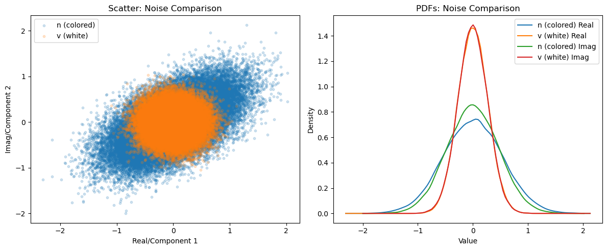
v_samples = W @ n_samples
plot_comparison(n_samples, v_samples, 'n (colored)', 'v (white)', 'Noise Comparison')
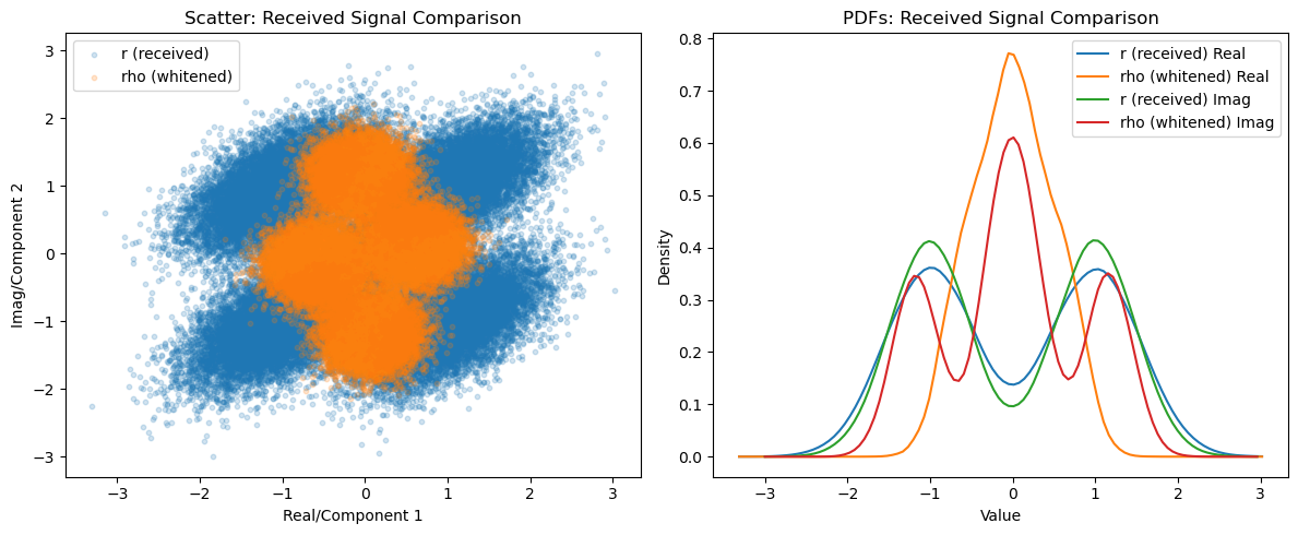
plot_comparison(r_samples, rho_samples, 'r (received)', 'rho (whitened)', 'Received Signal Comparison')
# Print BER values
print("Eb/N0 (dB) | BER (Colored) | BER (Whitened)")
for snr, bc, bw in zip(Eb_N0_dB_range, ber_colored, ber_whitened):
print(f"{snr:8d} | {bc:.6f} | {bw:.6f}")
Eb/N0 (dB) | BER (Colored) | BER (Whitened)
       0   | 0.159970    | 0.135340
       2   | 0.102530    | 0.082180
       4   | 0.056700    | 0.039330
       6   | 0.023190    | 0.012570
       8   | 0.006180    | 0.002110
      10   | 0.000960    | 0.000180
      12   | 0.000030    | 0.000000
      14   | 0.000000    | 0.000000
# Plot BER vs Eb/N0
plt.figure(figsize=(8, 6))
plt.semilogy(Eb_N0_dB_range, ber_colored, 'b-o', label='Colored Noise (r)')
plt.semilogy(Eb_N0_dB_range, ber_whitened, 'r-^', label='Whitened Noise (rho)')
plt.xlabel('Eb/N0 (dB)')
plt.ylabel('Bit Error Rate (BER)')
plt.title('BER vs Eb/N0: Colored vs Whitened Noise (Binary Sequence)')
plt.grid(True, which="both")
plt.legend()
plt.show()
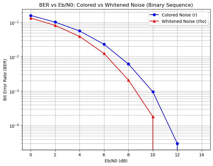
Due to the numerical mismatch, the whitened BER is not similar to AWGN BER in this simulation.