Detection Problem with Multiple Samples#
We consider a Detection Problem with Multiple (Discrete) Samples, where multiple discrete samples are utilized to decide between two hypotheses, \( H_0 \) and \( H_1 \).
Using multiple samples enhances decision-making accuracy by leveraging more information from several measurements.
By expanding the analysis to multiple samples, we can apply more sophisticated decision criteria and achieve better performance in distinguishing between the two hypotheses.
Real Measurement Samples:
Assume we have \( k \) real samples or measurements denoted by \( \mathbf{y}_1, \mathbf{y}_2, \ldots, \mathbf{y}_k \). Each \(\mathbf{y}_j\) represents a single measurement in the sequence.
Signal Samples:
For each hypothesis, there are \( k \) signal samples:
Under \( H_0 \): \( s_{0j} \) for \( j = 1, \ldots, k \)
Under \( H_1 \): \( s_{1j} \) for \( j = 1, \ldots, k \)
Measurement Sample Model#
The real measurements are modeled as:
where \(\mathbf{n}_j\): Random noise associated with the \( j \)-th sample.
So each measurement \( \mathbf{y}_j \) is the sum of the signal \( s_{ij} \) (depending on the hypothesis) and the noise \( \mathbf{n}_j \).
Discussion.
Despite having \( 2k \) possible signal samples, we only observe \( k \) real measurements \( \mathbf{y}_j \), where each \( \mathbf{y}_j \) is influenced by one of the two hypotheses.
Specifically, for each observation \( \mathbf{y}_j \), there are two possible signal contributions—one under \( H_0 \) and one under \( H_1 \).
However, only one of these hypotheses is true at any given time, meaning that for each \( \mathbf{y}_j \), only one signal sample (\( s_{0j} \) or \( s_{1j} \)) is actually contributing to the observation.
Complex Measurements#
For complex representations, the measurements are expressed as:
where:
\(\alpha\): Attenuation factor of the received signal.
\(\beta\): Phase shift of the received signal.
\( u_{i,j} \): \( j \)-th sample of the \( i \)-th baseband equivalent signal.
\(\mathbf{z}_j\): \( j \)-th sample of the baseband equivalent noise.
This complex model accounts for signal attenuation and phase changes in a complex baseband environment.
Vector Notation for Samples#
To streamline the notation when dealing with \( k \) samples, we define a column vector:
This vector aggregates all measurements into a single \( k \)-dimensional entity.
Conditional Probabilities#
The probabilities conditioned on each hypothesis are defined as:
where:
\( p_0(\vec{y}) \): Joint probability of observing the vector \( \vec{\mathbf{y}} \) under \( H_0 \).
\( p_1(\vec{y}) \): Joint probability of observing the vector \( \vec{\mathbf{y}} \) under \( H_1 \).
Decision Regions#
The decision process involves partitioning the \( k \)-dimensional sample space into two regions:
\( R_0 \): Region where decision \( D_0 \) (accepting \( H_0 \)) is made.
\( R_1 \): Region where decision \( D_1 \) (accepting \( H_1 \)) is made.
If the sample vector \( \vec{\mathbf{y}} \) falls within \( R_i \) (\( i = 0 \) or \( 1 \)), then the corresponding decision \( D_i \) is selected.
Discussion: k-Dimensional Decision Region
The decision is k-dimensional because it is based on k independent observations or measurements.
Each measurement contributes a separate dimension to the overall decision-making process.
Example of a k-Dimensional Decision Region#
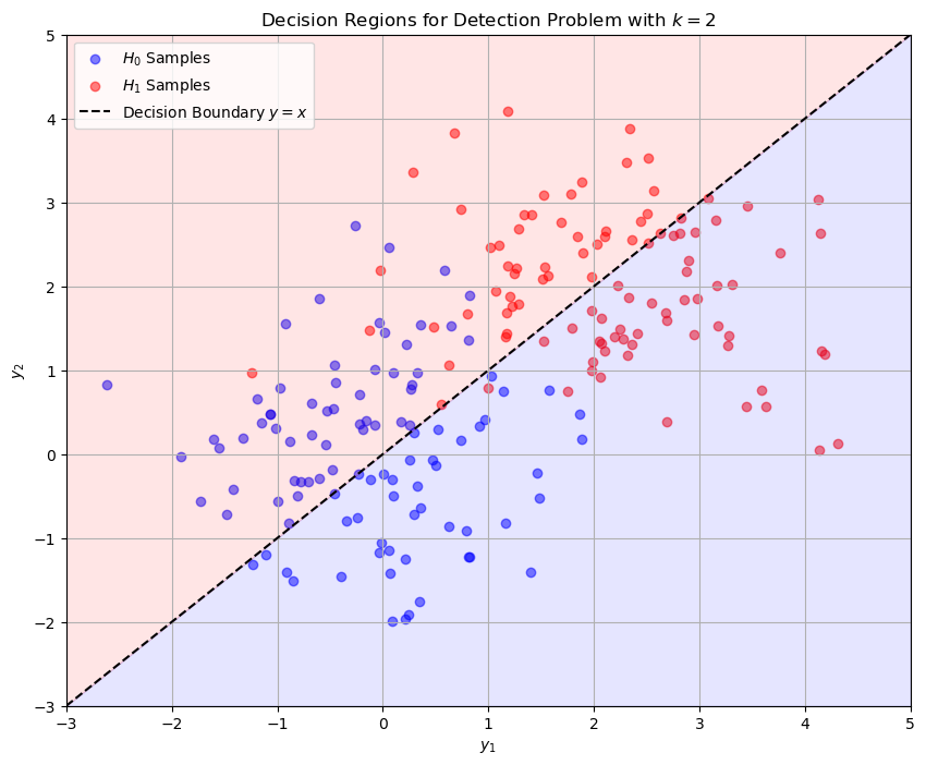
To illustrate this concept, we consider a simple case where \( k = 2 \).
This means we have two measurements, \( \mathbf{y}_1 \) and \( \mathbf{y}_2 \), forming a 2-dimensional sample vector \( \vec{\mathbf{y}} = [\mathbf{y}_1, \mathbf{y}_2]^T \).
Scenario Setup:
Hypotheses:
\( H_0 \): The measurements are centered around \( \vec{s}_0 = [s_{01}, s_{02}]^T \).
\( H_1 \): The measurements are centered around \( \vec{s}_1 = [s_{11}, s_{12}]^T \).
Noise:
Assume additive Gaussian noise with variance \( \sigma^2 \) in each dimension.
Thus, under each hypothesis, the observations are:
\[ \mathbf{y}_j = s_{ij} + \mathbf{n}_j, \quad i = 0, 1; \quad j = 1, 2 \]where \( \mathbf{n}_j \sim \mathcal{N}(0, \sigma^2) \).
Decision Boundary#
To decide between \( H_0 \) and \( H_1 \), we define a decision boundary that separates the two regions \( R_0 \) and \( R_1 \).
Linear Decision Boundary (Equal Priors and Variances):
If \( H_0 \) and \( H_1 \) have equal prior probabilities and noise variances, the decision boundary is the perpendicular bisector of the line segment connecting \( \vec{s}_0 \) and \( \vec{s}_1 \).
This boundary is a straight line where:
\[ (\vec{\mathbf{y}} - \vec{s}_0) \cdot (\vec{s}_1 - \vec{s}_0) = (\vec{s}_1 - \vec{s}_0) \cdot (\vec{s}_1 - \vec{s}_0)/2 \]Points on one side of the boundary belong to \( R_0 \), and points on the other side belong to \( R_1 \).
import numpy as np
import matplotlib.pyplot as plt

# Set random seed for reproducibility
np.random.seed(42)

# Parameters
k = 2  # Number of dimensions
num_samples = 100  # Number of samples per hypothesis
sigma = 1.0  # Standard deviation of noise

# Hypothesis means
s0 = np.array([0, 0])  # Mean under H0
s1 = np.array([2, 2])  # Mean under H1

# Generate samples under H0
noise_H0 = np.random.normal(0, sigma, (num_samples, k))
samples_H0 = s0 + noise_H0

# Generate samples under H1
noise_H1 = np.random.normal(0, sigma, (num_samples, k))
samples_H1 = s1 + noise_H1

# Plotting
plt.figure(figsize=(10, 8))

# Plot H0 samples
plt.scatter(samples_H0[:, 0], samples_H0[:, 1], color='blue', alpha=0.5, label='$H_0$ Samples')

# Plot H1 samples
plt.scatter(samples_H1[:, 0], samples_H1[:, 1], color='red', alpha=0.5, label='$H_1$ Samples')

# Decision boundary: y = x
x_vals = np.linspace(-3, 5, 100)
y_vals = x_vals
plt.plot(x_vals, y_vals, 'k--', label='Decision Boundary $y = x$')

# Shade decision regions
plt.fill_between(x_vals, -3, x_vals, color='blue', alpha=0.1)
plt.fill_between(x_vals, x_vals, 5, color='red', alpha=0.1)

# Labels and title
plt.title('Decision Regions for Detection Problem with $k=2$')
plt.xlabel('$y_1$')
plt.ylabel('$y_2$')
plt.legend()
plt.grid(True)
plt.xlim(-3, 5)
plt.ylim(-3, 5)
plt.show()

# Function to classify new observations
def classify(y, boundary_func):
    if boundary_func(y[0]) > y[1]:
        return 'H0'
    else:
        return 'H1'

# Example new observations
new_observations = np.array([
    [1, 0],
    [3, 4],
    [0, 1],
    [2, 2],
    [4, 1]
])

# Classify and plot new observations
plt.figure(figsize=(10, 8))

# Plot existing samples
plt.scatter(samples_H0[:, 0], samples_H0[:, 1], color='blue', alpha=0.5, label='$H_0$ Samples')
plt.scatter(samples_H1[:, 0], samples_H1[:, 1], color='red', alpha=0.5, label='$H_1$ Samples')

# Decision boundary
plt.plot(x_vals, y_vals, 'k--', label='Decision Boundary $y = x$')

# Shade decision regions
plt.fill_between(x_vals, -3, x_vals, color='blue', alpha=0.1)
plt.fill_between(x_vals, x_vals, 5, color='red', alpha=0.1)

# Classify and plot new observations
for obs in new_observations:
    decision = classify(obs, lambda x: x)  # y = x boundary
    if decision == 'H0':
        plt.scatter(obs[0], obs[1], color='blue', edgecolors='k', marker='o', s=100, label='New $H_0$' if 'H0_label' not in locals() else "")
        locals()['H0_label'] = True
    else:
        plt.scatter(obs[0], obs[1], color='red', edgecolors='k', marker='s', s=100, label='New $H_1$' if 'H1_label' not in locals() else "")

# Labels and title
plt.title('Classification of New Observations')
plt.xlabel('$y_1$')
plt.ylabel('$y_2$')
plt.legend()
plt.grid(True)
plt.xlim(-3, 5)
plt.ylim(-3, 5)
plt.show()

# Print classification results
for i, obs in enumerate(new_observations):
    decision = classify(obs, lambda x: x)
    print(f"Observation {i+1}: {obs} classified as {decision}")


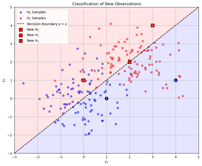
Observation 1: [1 0] classified as H0
Observation 2: [3 4] classified as H1
Observation 3: [0 1] classified as H1
Observation 4: [2 2] classified as H1
Observation 5: [4 1] classified as H0
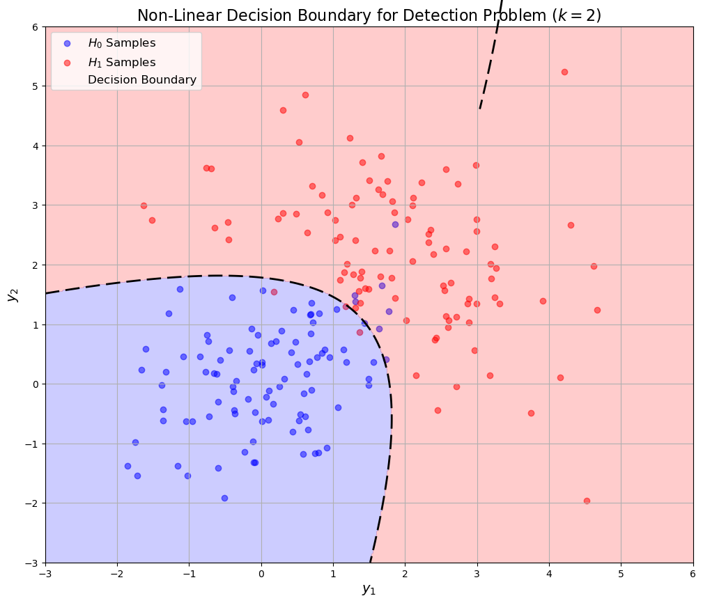
Non-linear Decision Boundary Example#
import numpy as np
import matplotlib.pyplot as plt
from scipy.stats import multivariate_normal
import warnings

# Suppress warnings for cleaner output
warnings.filterwarnings('ignore')

# Set random seed for reproducibility
np.random.seed(42)

# -------------------------
# 1. Parameters Setup
# -------------------------
k = 2  # Number of dimensions
num_samples = 100  # Number of samples per hypothesis

# Hypothesis parameters
# H0
s0 = np.array([0, 0])
Sigma0 = np.array([[1, 0.5],
                   [0.5, 1]])

# H1
s1 = np.array([2, 2])
Sigma1 = np.array([[1.5, -0.5],
                   [-0.5, 1.5]])

# -------------------------
# 2. Data Generation
# -------------------------
# Generate samples under H0
samples_H0 = np.random.multivariate_normal(s0, Sigma0, num_samples)

# Generate samples under H1
samples_H1 = np.random.multivariate_normal(s1, Sigma1, num_samples)

# -------------------------
# 3. Decision Boundary Computation
# -------------------------
# Define grid for plotting decision boundary
x_min, x_max = -3, 6
y_min, y_max = -3, 6
grid_size = 500  # Increased grid size for smoother boundary
xx, yy = np.meshgrid(np.linspace(x_min, x_max, grid_size),
                     np.linspace(y_min, y_max, grid_size))
grid = np.c_[xx.ravel(), yy.ravel()]

# Compute LLR for each point in the grid
# Assuming equal priors and using log-likelihood ratio
rv0 = multivariate_normal(s0, Sigma0)
rv1 = multivariate_normal(s1, Sigma1)

# Compute log-likelihoods
log_likelihood_ratio = rv1.logpdf(grid) - rv0.logpdf(grid)

# Reshape for contour plotting
log_likelihood_ratio = log_likelihood_ratio.reshape(xx.shape)

# -------------------------
# 4. Plotting Decision Boundary and Regions
# -------------------------
plt.figure(figsize=(12, 10))

# Plot H0 samples
plt.scatter(samples_H0[:, 0], samples_H0[:, 1],
            color='blue', alpha=0.5, label='$H_0$ Samples')

# Plot H1 samples
plt.scatter(samples_H1[:, 0], samples_H1[:, 1],
            color='red', alpha=0.5, label='$H_1$ Samples')

# Plot decision boundary using contour where LLR=0
contour = plt.contour(xx, yy, log_likelihood_ratio, levels=[0],
                     colors='k', linestyles='--', linewidths=2)
contour.collections[0].set_label('Decision Boundary')

# Shade decision regions
# Use two distinct colors with transparency for better visibility
plt.contourf(xx, yy, log_likelihood_ratio > 0, alpha=0.2,
             colors=['blue', 'red'])

# -------------------------
# 5. Plot Formatting
# -------------------------
# Labels and title
plt.title('Non-Linear Decision Boundary for Detection Problem ($k=2$)', fontsize=16)
plt.xlabel('$y_1$', fontsize=14)
plt.ylabel('$y_2$', fontsize=14)

# Custom legend to avoid duplicate labels
handles, labels = plt.gca().get_legend_handles_labels()
by_label = dict(zip(labels, handles))
plt.legend(by_label.values(), by_label.keys(), fontsize=12)

plt.grid(True)
plt.xlim(x_min, x_max)
plt.ylim(y_min, y_max)
plt.show()

# -------------------------
# 6. Classification Function
# -------------------------
def classify_lrt(y, rv0, rv1):
    """
    Classify a new observation based on the log-likelihood ratio.

    Parameters:
    - y: numpy array of shape (2,)
    - rv0: scipy.stats.multivariate_normal object for H0
    - rv1: scipy.stats.multivariate_normal object for H1

    Returns:
    - 'H0' or 'H1'
    """
    return 'H1' if rv1.logpdf(y) > rv0.logpdf(y) else 'H0'

# -------------------------
# 7. New Observations Classification and Plotting
# -------------------------
# Example new observations
new_observations = np.array([
    [1, 0],
    [3, 4],
    [0, 1],
    [2, 2],
    [4, 1],
    [1.5, 1.5],
    [2.5, 0.5]
])

# Classify and plot new observations
plt.figure(figsize=(12, 10))

# Plot existing samples
plt.scatter(samples_H0[:, 0], samples_H0[:, 1],
            color='blue', alpha=0.5, label='$H_0$ Samples')
plt.scatter(samples_H1[:, 0], samples_H1[:, 1],
            color='red', alpha=0.5, label='$H_1$ Samples')

# Plot decision boundary
contour = plt.contour(xx, yy, log_likelihood_ratio, levels=[0],
                     colors='k', linestyles='--', linewidths=2)
contour.collections[0].set_label('Decision Boundary')

# Shade decision regions
plt.contourf(xx, yy, log_likelihood_ratio > 0, alpha=0.2,
             colors=['blue', 'red'])

# Track labels to prevent duplicates
label_added_H0 = False
label_added_H1 = False

# Classify and plot new observations
for i, obs in enumerate(new_observations):
    decision = classify_lrt(obs, rv0, rv1)
    if decision == 'H0' and not label_added_H0:
        plt.scatter(obs[0], obs[1], color='blue',
                    edgecolors='k', marker='o', s=100,
                    label='New $H_0$')
        label_added_H0 = True
    elif decision == 'H1' and not label_added_H1:
        plt.scatter(obs[0], obs[1], color='red',
                    edgecolors='k', marker='s', s=100,
                    label='New $H_1$')
        label_added_H1 = True
    elif decision == 'H0':
        plt.scatter(obs[0], obs[1], color='blue',
                    edgecolors='k', marker='o', s=100)
    else:
        plt.scatter(obs[0], obs[1], color='red',
                    edgecolors='k', marker='s', s=100)

# Labels and title
plt.title('Classification of New Observations with Non-Linear Decision Boundary', fontsize=16)
plt.xlabel('$y_1$', fontsize=14)
plt.ylabel('$y_2$', fontsize=14)

# Custom legend to avoid duplicate labels
handles, labels = plt.gca().get_legend_handles_labels()
by_label = dict(zip(labels, handles))
plt.legend(by_label.values(), by_label.keys(), fontsize=12)

plt.grid(True)
plt.xlim(x_min, x_max)
plt.ylim(y_min, y_max)
plt.show()

# -------------------------
# 8. Print Classification Results
# -------------------------
print("=== Classification Results ===")
for i, obs in enumerate(new_observations):
    decision = classify_lrt(obs, rv0, rv1)
    print(f"Observation {i+1}: {obs} classified as {decision}")


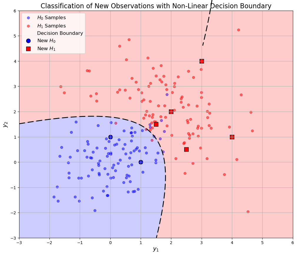
=== Classification Results ===
Observation 1: [1. 0.] classified as H0
Observation 2: [3. 4.] classified as H1
Observation 3: [0. 1.] classified as H0
Observation 4: [2. 2.] classified as H1
Observation 5: [4. 1.] classified as H1
Observation 6: [1.5 1.5] classified as H1
Observation 7: [2.5 0.5] classified as H1
Examples of Multiple Measurements#
Multiple samples or measurements are fundamental in enhancing the accuracy and reliability of decision-making processes.
These measurements can originate from various domains, each offering unique advantages and applications.
Additionally, hybrid scenarios combining two or more of these measurement types are common, leveraging the strengths of each method to achieve optimal results.
Time#
Time-based measurements are prevalent in many engineering and scientific applications, especially within communication systems. Here’s an in-depth look at how multiple time samples are utilized:
Continuous Signals in Communication Systems:
In communication systems, data is often transmitted using continuous-time signals. Consider two possible noise-free, continuous signals represented as:
where:
\( s_i(t) \): Represents one of the two possible real-valued signals under hypotheses \( H_0 \) and \( H_1 \).
\( u_i(t) \): Complex baseband signal corresponding to each hypothesis.
\( f_c \): Carrier frequency.
\( \Re \): Denotes the real part of the complex expression.
Observation with Noise:
The received signal in the presence of noise is modeled as:
where:
\( \mathbf{y}(t) \): Real measurement at time \( t \).
\( \mathbf{n}(t) \): Additive noise, typically modeled as a random process (e.g., Gaussian noise).
Time Sampling:
Sampling the continuous signal \( \mathbf{y}(t) \) at discrete time instances \( t_1, t_2, \ldots, t_k \) results in multiple discrete measurements:
Multiple Measurements Model: Each \( \mathbf{y}_j \) is a separate observation influenced by the underlying hypothesis \( H_i \) and noise.
Discrete-Time Systems:
Modern communication systems often operate in discrete-time for easier processing and implementation.
This discretization simplifies the measurement model and facilitates digital signal processing techniques.
Example Scenario:
Imagine a digital communication system where binary data is transmitted using two distinct waveforms corresponding to \( H_0 \) (bit 0) and \( H_1 \) (bit 1).
The receiver samples the incoming signal at multiple time instances to determine the transmitted bit by comparing the sequence of received samples against the expected signal patterns.
Frequency#
Frequency-based measurements involve analyzing signals at different frequency bands, which is especially useful in environments where signal characteristics vary with frequency.
Frequency Sampling in Communication:
Instead of or in addition to time-domain sampling, signals can be sampled across various frequencies.
This approach is beneficial in scenarios where signal attenuation or fading varies with frequency.
Radio Communication and Fading Channels:
Radio channels often experience fading, where signal strength fluctuates due to factors like multipath propagation and interference.
These fluctuations can vary across different frequency bands.
To mitigate this, information is transmitted simultaneously across multiple frequency bands:
where:
\( \mathbf{y}_j \): Received signal sample at the \( j \)-th frequency band.
\( \boldsymbol{\alpha}_j \): Random variable representing signal attenuation in the \( j \)-th band.
\( \boldsymbol{\beta}_j \): Phase random variable in the \( j \)-th band.
\( u_{i,j} \): Baseband equivalent signal component under hypothesis \( H_i \).
\( \mathbf{z}_j \): Noise in the \( j \)-th frequency band.
Advantages of Frequency Sampling:
Diversity Gain: By transmitting over multiple frequencies, the probability that all channels experience deep fading simultaneously is reduced.
Enhanced Reliability: Multiple frequency channels provide redundancy, ensuring that even if some channels are compromised, others maintain signal integrity.
Radio Astronomy Applications:
In radio astronomy, observing celestial sources across multiple frequencies allows astronomers to construct a comprehensive spectral profile of the source.
This multi-frequency analysis provides insights into the physical properties and behaviors of astronomical objects.
Example Scenario:
A radio transmitter sends the same information across three different frequency bands to a receiver.
Each band may experience different levels of attenuation and phase shifts due to environmental factors.
By combining the information from all three bands, the receiver can more accurately reconstruct the original signal, ensuring reliable communication despite channel impairments.
Spatial#
Spatial measurements involve using multiple sensors or detectors distributed across different physical locations.
This technique is widely used in communication, radar, and satellite systems to enhance signal detection and reliability. Here’s a detailed exploration:
Multiple Detectors in Communication and Radar Systems:
Deploying several detector circuits at various locations helps in capturing signals that might be attenuated or distorted due to environmental factors like rain, terrain, or obstacles.
Satellite Communication Example:
Consider radio signals transmitted from a satellite to the ground. These signals can suffer from severe attenuation caused by local rain.
To counteract this, multiple ground receivers are strategically placed:
where:
\( \mathbf{y}_{j\ell} \): Received signal at the \( \ell \)-th receiver for the \( j \)-th measurement.
\( \boldsymbol{\alpha}_{j\ell} \): Attenuation factor for the \( j \)-th measurement at the \( \ell \)-th receiver.
\( \boldsymbol{\beta}_{j\ell} \): Phase shift for the \( j \)-th measurement at the \( \ell \)-th receiver.
\( u_{i,j} \): Baseband equivalent signal under hypothesis \( H_i \) for the \( j \)-th measurement.
\( \mathbf{z}_{j\ell} \): Noise at the \( \ell \)-th receiver for the \( j \)-th measurement.
\( D \): Total number of ground receivers.
Advantages of Spatial Diversity:
Redundancy: Multiple receivers ensure that if one or more are affected by adverse conditions (e.g., heavy rain), others can still capture the signal effectively.
Improved Signal Quality: Combining signals from multiple receivers can enhance the overall signal-to-noise ratio (SNR), leading to better detection and decoding performance.
Receiver Placement Considerations:
Receivers are typically spaced kilometers apart to minimize the likelihood that multiple receivers are simultaneously impacted by the same adverse event (e.g., an intense rain cell).
This spatial separation ensures that the probability of multiple signal losses is significantly reduced.
Example Scenario:
A satellite communication system employs five ground receivers located in different geographic areas.
Each receiver independently captures the satellite’s signal, which may be attenuated differently due to local weather conditions.
The system aggregates the data from all receivers to reconstruct the transmitted information reliably, ensuring continuous communication even if some receivers experience signal degradation.
Hybrid Measurements#
In real-world applications, it’s common to encounter hybrid scenarios that combine two or more of the aforementioned measurement types. For instance:
Time-Frequency Sampling:
A communication system might employ both time-based and frequency-based sampling to exploit temporal diversity and frequency diversity simultaneously.
This approach enhances robustness against both time-varying noise and frequency-selective fading.
Time-Spatial Sampling:
In radar systems, multiple spatially distributed detectors might capture reflections of a signal over time, providing comprehensive spatiotemporal data for accurate target detection and tracking.
Frequency-Spatial Sampling:
In radio astronomy, observations across multiple frequencies and spatial locations enable astronomers to create detailed maps of celestial sources, capturing both spectral and spatial information.
Significance of Hybrid Measurements:
Enhanced Reliability: Combining different measurement modalities reduces the likelihood of simultaneous signal loss across all channels.
Comprehensive Data Analysis: Hybrid measurements provide a richer dataset, allowing for more sophisticated analysis and improved decision-making.
Flexibility: Systems can adapt to varying environmental conditions by leveraging multiple measurement types to maintain performance.
MATLAB Example: Detect Human Presence Using Wireless Sensing with Deep Learning
