Signal Representations

Real Signals

Real Lowpass Signal

Definition: Bandwidth
For a real signal \(x(t)\), the bandwidth is the smallest range of positive frequencies such that \(X(f) = 0\) when \(|f|\) lies outside this range.
It follows that the bandwidth of a real signal is half of its total frequency support.

Definition: Lowpass (or Baseband) Signal
A lowpass or baseband signal is one whose spectrum is concentrated around the zero frequency.

For instance, speech, music, and video signals are examples of lowpass signals, even though they differ in spectral characteristics and bandwidths. Typically, lowpass signals are low-frequency signals, meaning they vary slowly over time and do not exhibit sudden jumps or rapid changes.

The bandwidth of a real lowpass signal is the smallest positive value \(W\) such that \(X(f) = 0\) for all frequencies outside the range \([-W, +W]\).

Additional Notes on Bandwidth and Complex Signals

• The spectrum of a real signal can be expressed as:

  \[ X(f) = X_+(f) + X_-(f) \]

  where:

  • \(X_+(f) = X(f) \cdot u_{-1}(f)\) (the positive-frequency component)

  • \(X_-(f) = X(f) \cdot u_{-1}(-f)\) (the negative-frequency component)

• For a complex signal \(x(t)\), the spectrum \(X(f)\) is not symmetric, meaning the signal cannot be reconstructed using only positive-frequency information.

Definition: Bandwidth of Complex Signals
For a complex signal, the bandwidth is defined as half of the entire range of frequencies over which the spectrum is nonzero. This corresponds to half of the signal’s frequency support.

This definition ensures consistency with the bandwidth definition for real signals. Thus, for both real and complex signals, the bandwidth is defined as half of the frequency support.

Bandpass Signals

Motivation for Using Bandpass Signals

• In practice, the spectral characteristics of the message signal and the communication channel often do not align.

• To address this mismatch, the message signal is modulated to match its spectral characteristics to those of the channel.

By modulating the lowpass message signal, its spectrum is shifted to higher frequencies, resulting in a bandpass signal.

Definition and Characteristics

A bandpass signal is a real signal whose frequency content (spectrum) is concentrated around a frequency \( \pm f_0 \), which is far from zero.

Definition: Bandpass Signal
A bandpass signal is a real signal \( x(t) \) for which there exist positive \( f_0 \) and \( W \) such that the positive spectrum \( X_+(f) \) is nonzero only within the interval \([f_0 - W/2, f_0 + W/2]\), where \( W/2 < f_0 \) (in practice, \( W \ll f_0 \)).

Definition: Central Frequency
The frequency \( f_0 \) is referred to as the central frequency of the bandpass signal.

Key Points:

• The bandwidth of \( x(t) \) is at most \( W \).

• Bandpass signals are typically high-frequency signals characterized by rapid variations in the time domain.

Spectrum of a Bandpass Signal

Figure: Spectrum of a Real-Valued Bandpass Signal
The spectrum of a real bandpass signal is shown below.

• The magnitude spectrum (solid line) is even.

• The phase spectrum (dashed line) is odd.

• The central frequency \( f_0 \) is not necessarily the midband frequency of the bandpass signal.

Symmetry and Reconstruction:

• Since \( x(t) \) is a real signal, the spectrum \( X(f) \) exhibits symmetry.

• The positive spectrum \( X_+(f) \) contains all the necessary information to reconstruct \( X(f) \):

  \[ X(f) = X_+(f) + X_-(f) = X_+(f) + X_+^*(-f) \]

  This means that knowledge of \( X_+(f) \) is sufficient to fully determine \( X(f) \).

Python Simulation

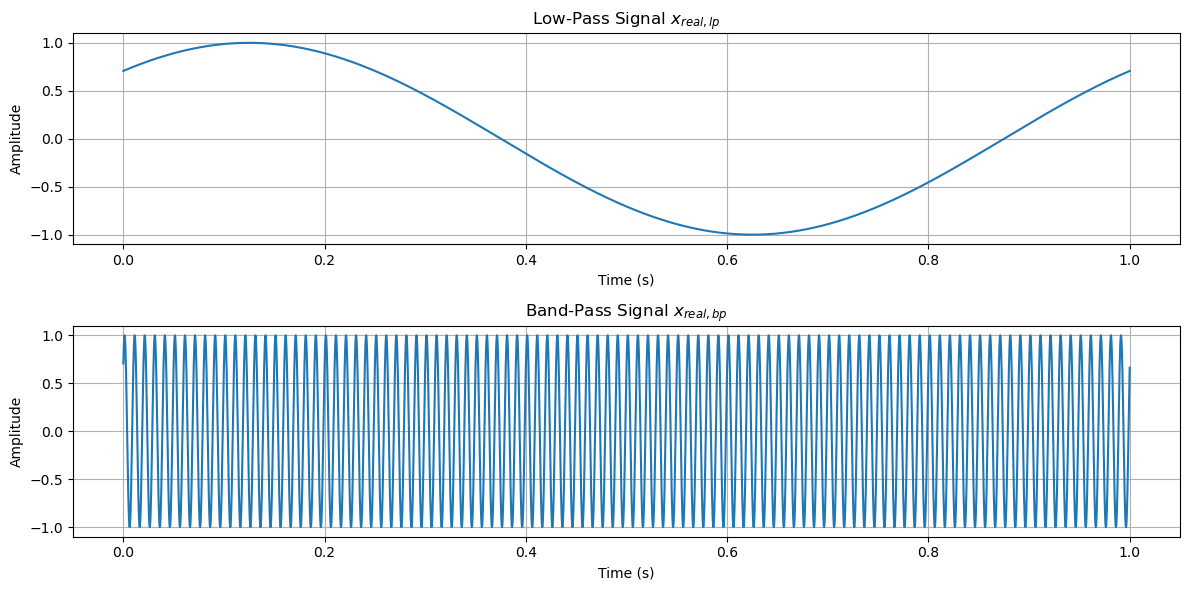
Low-Pass Signal:
The low-pass signal is generated as:

\[ x_{\text{real,lp}}(t) = a \cdot \sin(\omega_0 \cdot t + \theta) \]

where:

• \( \omega_0 = \frac{2\pi}{T} \) is the baseband angular frequency, corresponding to a frequency \( f_0 = \frac{1}{T} \) Hz.

• In this example, \( T = 1 \), so \( f_0 = 1 \) Hz.

This means the low-pass signal has a sinusoidal frequency content at \( f_0 = 1 \) Hz, which is close to 0 Hz in the spectrum.

import numpy as np
import matplotlib.pyplot as plt

# Define parameters
a = 1                   # Amplitude
T = 1                   # Signal period (seconds)
fs = 10000               # Sampling rate (samples per second)
omega_0 = 2 * np.pi / T # Baseband angular frequency (rad/s)
f_c = 100               # Carrier frequency (Hz)
theta = np.pi / 4       # Phase in radians

# Time vector: compute based on signal period and sampling rate
t = np.arange(0, T, 1/fs)  # Time vector from 0 to T seconds with 1/fs interval

# Generate the low-pass signal
x_real_lp = a * np.sin(omega_0 * t + theta)

# Generate the band-pass signal
omega_c = 2 * np.pi * f_c  # Convert carrier frequency to angular frequency
x_real_bp = a * np.sin(omega_c * t + theta)

# Plot the signals
plt.figure(figsize=(12, 6))

# Plot low-pass signal
plt.subplot(2, 1, 1)
plt.plot(t, x_real_lp)
plt.title('Low-Pass Signal $x_{real, lp}$')
plt.xlabel('Time (s)')
plt.ylabel('Amplitude')
plt.grid(True)

# Plot band-pass signal
plt.subplot(2, 1, 2)
plt.plot(t, x_real_bp)
plt.title('Band-Pass Signal $x_{real, bp}$')
plt.xlabel('Time (s)')
plt.ylabel('Amplitude')
plt.grid(True)

# Show the plots
plt.tight_layout()
plt.show()

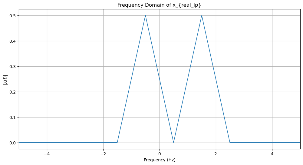
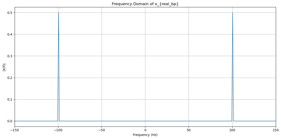
Fourier Transform:

• The FT of a sinusoidal signal results in two impulses at the positive and negative frequency of the signal:

  • \( \pm f_0 = \pm 1 \) Hz.

• Since this is a low-pass signal, the FT is concentrated near the center of the spectrum (0 Hz).

Frequency Vector and FFT Output:

• The frequency vector f is centered at 0 (using np.fft.fftshift), so the FT of the low-pass signal will appear symmetrically around 0 Hz, with peaks at \( \pm 1 \) Hz.

# Compute the FFT of the low-pass signal
X_real_lp_fft_shifted = np.fft.fftshift(np.fft.fft(x_real_lp))  # Compute and shift FFT
X_real_bp_fft_shifted = np.fft.fftshift(np.fft.fft(x_real_bp))  # Compute and shift FFT

# Frequency vector
N = len(t)                      # Total number of samples
f = np.linspace(-fs/2, fs/2, N) # Frequency vector in Hz, centered at 0
# Plot the signals


# Plot low-pass signal in the frequency domain
plt.figure(figsize=(12, 6))
plt.plot(f, np.abs(X_real_lp_fft_shifted)/N, linewidth=1.2)
plt.title('Frequency Domain of x_{real_lp}')
plt.xlabel('Frequency (Hz)')
plt.ylabel('|X(f)|')
plt.xlim([-5, 5]) # Limit frequency axis for low-pass signal
plt.grid(True)

# Plot band-pass signal in the frequency domain
plt.figure(figsize=(12, 6))
plt.plot(f, np.abs(X_real_bp_fft_shifted)/N, linewidth=1.2)
plt.title('Frequency Domain of x_{real_bp}')
plt.xlabel('Frequency (Hz)')
plt.ylabel('|X(f)|')
plt.xlim([-150, 150]) # Limit frequency axis for band-pass signal
plt.grid(True)

# Adjust layout for better visualization
plt.tight_layout()
plt.show()

import numpy as np
import matplotlib.pyplot as plt

# Define parameters
a = 1                   # Amplitude
T = 1                   # Signal period (seconds)
fs = 1000               # Sampling rate (samples per second)
omega_0 = 2 * np.pi / T # Baseband angular frequency (rad/s)
theta = np.pi / 4       # Phase in radians

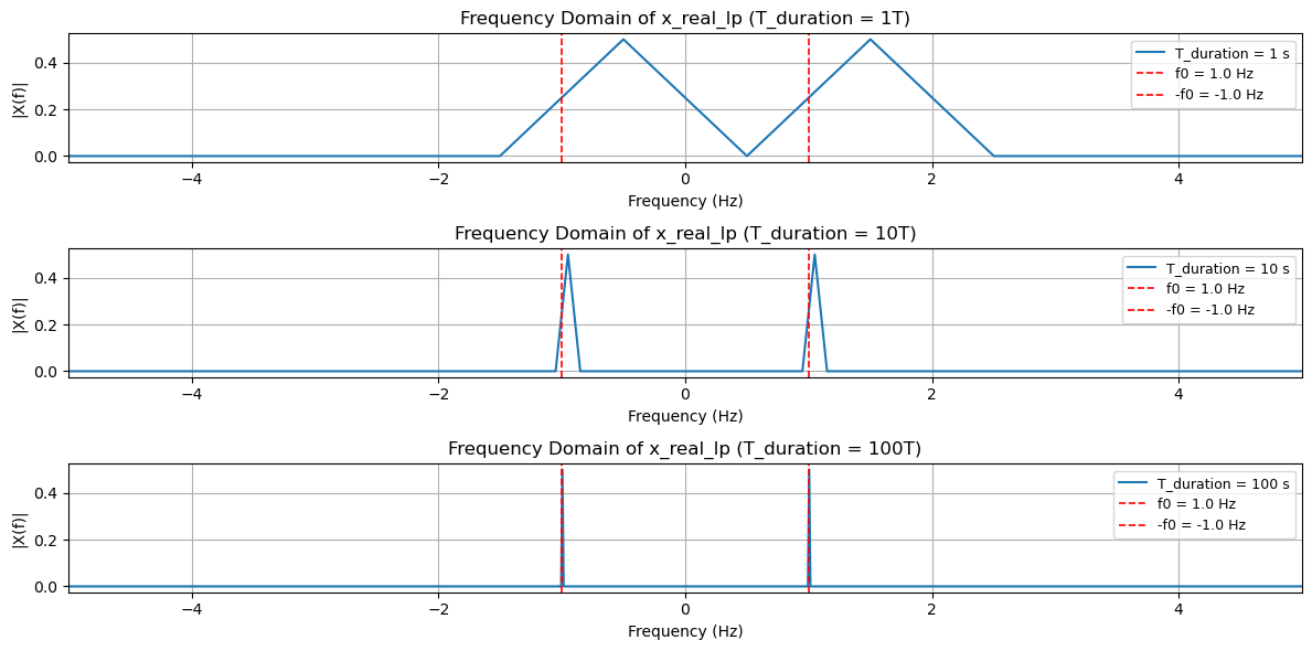
# Different T_duration values
T_durations = [1 * T, 10 * T, 100 * T]

# Create a figure
plt.figure(figsize=(12, 6))

# Loop over different T_duration values
for i, T_duration in enumerate(T_durations):
    # Time vector and signal length
    t = np.arange(0, T_duration, 1/fs)
    N = len(t)  # Total number of samples

    # Regenerate the low-pass signal
    x_real_lp = a * np.sin(omega_0 * t + theta)

    # Compute the FFT and frequency vector
    X_real_lp_fft_shifted = np.fft.fftshift(np.fft.fft(x_real_lp))
    f = np.linspace(-fs/2, fs/2, N)

    # Plot the Fourier Transform
    plt.subplot(3, 1, i + 1)  # Create a subplot for each T_duration
    plt.plot(f, np.abs(X_real_lp_fft_shifted)/N, linewidth=1.5, label=f'T_duration = {T_duration} s')
    plt.axvline(x=1/T, color='red', linestyle='--', linewidth=1.2, label=f'f0 = {1/T} Hz')  # Positive f0
    plt.axvline(x=-1/T, color='red', linestyle='--', linewidth=1.2, label=f'-f0 = {-1/T} Hz')  # Negative f0
    plt.title(f'Frequency Domain of x_real_lp (T_duration = {T_duration:.0f}T)', fontsize=12)
    plt.xlabel('Frequency (Hz)', fontsize=10)
    plt.ylabel('|X(f)|', fontsize=10)
    plt.xlim([-5, 5])  # Limit frequency axis for better visualization
    plt.grid(True)
    plt.legend(fontsize=9)

# Adjust layout for better visualization
plt.tight_layout()
plt.show()

Analytic Signal (Pre-envelope)

Definition: Analytic Signal
The analytic signal (also called the pre-envelope) corresponding to a signal \(x(t)\) is the complex signal \(x_+(t)\) whose Fourier transform is \(X_+(f)\). It is defined as:

\[ x_+(t) = \mathcal{F}^{-1}[X_+(f)] = \frac{1}{2}x(t) + j\frac{1}{2}\hat{x}(t) \]

Here, \(\hat{x}(t)\) is the Hilbert transform of \(x(t)\), given by:

\[ \hat{x}(t) = \frac{1}{\pi t} * x(t) \]

Hilbert Transform

The Hilbert transform of \(x(t)\):

• Introduces a phase shift of \(-\frac{\pi}{2}\) to the positive frequency components of \(x(t)\).

• Introduces a phase shift of \(+\frac{\pi}{2}\) to the negative frequency components of \(x(t)\).

In the frequency domain, it is expressed as:

\[ \mathcal{F}[\hat{x}(t)] = -j \, \text{sgn}(f) X(f) \]

Properties of the Analytic Signal

1. The analytic signal \(x_+(t)\) contains only positive frequency components.

2. Its spectrum \(X_+(f)\) is not Hermitian (i.e., it is not symmetric about the origin).

3. \(x_+(t)\) is generally a complex signal, even if \(x(t)\) is real.

Matlab Example: Compute Envelope Spectrum

Compute the envelope of the filtered signal using Hilbert as the method

Compute Envelope Spectrum of Vibration Signal