MAP Estimation for a Discrete Linear Observation Model#
The signal model described in previous section is continued in this section, i.e.,
However, it is assumed here that the parameter vector is random, independent of the noise \(\vec{n}\), and with a Gaussian pdf represented as
where \(\vec{\mu}_{\alpha}\) and \(A_{\alpha}\) are the mean and covariance matrix, respectively, of \(\vec{\alpha}\).
MAP Estimation#
A MAP estimate can be obtained for the vector \(\vec{\alpha}\) by computing
or in vector notation
The first term in this equation is computed as part of the ML estimate and is given by
The second term is determined from the matrix identity
where \(\vec{C}_v\) is a \(k\)-element real vector of constants.
With this identity, the second term becomes
since \((A_{\alpha}^{-1})^T = A_{\alpha}^{-1}\).
Combining these step, we have
The solution of this equation for \(\vec{\alpha}\) yields the MAP estimator
Note that the a posteriori pdf \(p(\vec{\alpha} | \vec{y})\) is Gaussian, so that the MAP and MSE estimates are the same.
Unbiased#
Using \(\mathbb{E}[\vec{y}] = \mathbb{E}[H \vec{\alpha}] = H \vec{\mu}_{\alpha}\), it can be seen that \(\vec{\hat{\alpha}}_{MAP}\) is unbiased.
That is:
Example#
A numerical example [B2, Ex. 12.4] is provided to illustrate the nature of the computations.
Assume that the observables are related by
where
Then, the following results can be obtained:
From which it follows that
From Eq. (12.46) and the previous relationships, the MAP estimate is
or
Simulation#
We have that
Write the MAP equations in matrix form (combine the terms involving \( y_1 \) and \( y_2 \) into a matrix multiplication, and separate the constant terms)
Define the components:
import numpy as np
import matplotlib.pyplot as plt


# Number of simulations
num_simulations = 100

# Define prior parameters
mu_alpha = np.array([1.0, 0.0, 0.0])  # mu_alpha = [1, 0, 0]
A_alpha = np.array([
    [2, 1, 0],
    [1, 2, 1],
    [0, 1, 1]
])

# Compute the inverse of A_alpha
A_alpha_inv = np.linalg.inv(A_alpha)

# Define noise covariance matrix R_n and its inverse R_n_inv
R_n = np.array([
    [2, 1],
    [1, 1]
])
R_n_inv = np.linalg.inv(R_n)

# Define H matrix
H = np.array([
    [1, 0, 1],
    [1, 1, 0]
])

# Precompute H^T R_n_inv
Ht_Rn_inv = H.T @ R_n_inv  # Shape: (3, 2)

# Compute H^T R_n_inv H + A_alpha_inv
Ht_Rn_H = Ht_Rn_inv @ H  # Shape: (3, 3)
Ht_Rn_H_plus_Ainv = Ht_Rn_H + A_alpha_inv  # Shape: (3, 3)

# Compute the inverse of (H^T Rn^{-1} H + A_alpha^{-1})
Ht_Rn_H_plus_Ainv_inv = np.linalg.inv(Ht_Rn_H_plus_Ainv)  # Shape: (3, 3)

# Compute the MAP estimator matrix
# This involves multiplying (Ht_Rn_H + Ainv)^{-1} with (Ht_Rn_inv)
MAP_estimator_matrix = Ht_Rn_H_plus_Ainv_inv @ Ht_Rn_inv  # Shape: (3, 2)

# Compute the term (Ht_Rn_H + Ainv)^{-1} A_alpha_inv mu_alpha
MAP_estimator_offset = Ht_Rn_H_plus_Ainv_inv @ A_alpha_inv @ mu_alpha  # Shape: (3,)

# Initialize arrays to store true and estimated parameters
true_alpha = np.random.multivariate_normal(mean=mu_alpha, cov=A_alpha, size=num_simulations)  # Shape: (num_simulations, 3)
alpha_estimates = np.zeros((num_simulations, 3))  # Columns: alpha1_est, alpha2_est, alpha3_est

# Perform simulations
for i in range(num_simulations):
    # Current true alpha vector
    alpha_current = true_alpha[i]

    # Generate noise sample from multivariate normal distribution
    noise = np.random.multivariate_normal(mean=np.zeros(2), cov=R_n)  # [n1, n2]

    # Generate measurements y1 and y2
    y = H @ alpha_current + noise  # Shape: (2,)

    # Compute MAP estimates
    alpha_map = MAP_estimator_matrix @ y + MAP_estimator_offset  # Shape: (3,)

    # Store estimates
    alpha_estimates[i] = alpha_map

# Compute statistics
alpha_estimates_mean = np.mean(alpha_estimates, axis=0)
alpha_estimates_std = np.std(alpha_estimates, axis=0)

# Cramér-Rao Bounds (CRB)
# The posterior covariance matrix is (H^T Rn^{-1} H + A_alpha^{-1})^{-1}
posterior_covariance = Ht_Rn_H_plus_Ainv_inv  # Shape: (3,3)
CRB_variances = np.diag(posterior_covariance)  # Variances for alpha1, alpha2, alpha3

# Display results
print("True Parameters Prior:")
print(f"mu_alpha = {mu_alpha}")
print(f"A_alpha =\n{A_alpha}\n")

print("MAP Estimator Results (Mean ± Std Dev):")
print(f"alpha1_est = {alpha_estimates_mean[0]:.4f} ± {alpha_estimates_std[0]:.4f}")
print(f"alpha2_est = {alpha_estimates_mean[1]:.4f} ± {alpha_estimates_std[1]:.4f}")
print(f"alpha3_est = {alpha_estimates_mean[2]:.4f} ± {alpha_estimates_std[2]:.4f}\n")

print("Cramér-Rao Bounds (CRB):")
print(f"Var(alpha1) >= {CRB_variances[0]:.4f}")
print(f"Var(alpha2) >= {CRB_variances[1]:.4f}")
print(f"Var(alpha3) >= {CRB_variances[2]:.4f}\n")

# Visualization

# Create an array of indices
indices = np.arange(1, num_simulations + 1)

# Select a subset of indices for clearer plots (e.g., first 1000)
plot_subset = 1000
subset_indices = indices[:plot_subset]
subset_true_alpha1 = true_alpha[:plot_subset, 0]
subset_true_alpha2 = true_alpha[:plot_subset, 1]
subset_true_alpha3 = true_alpha[:plot_subset, 2]
subset_est_alpha1 = alpha_estimates[:plot_subset, 0]
subset_est_alpha2 = alpha_estimates[:plot_subset, 1]
subset_est_alpha3 = alpha_estimates[:plot_subset, 2]

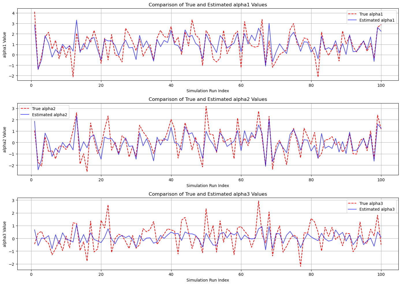
# Plot for alpha1
plt.figure(figsize=(14, 10))

plt.subplot(3, 1, 1)
plt.plot(subset_indices, subset_true_alpha1, label='True alpha1', color='red', linestyle='--')
plt.plot(subset_indices, subset_est_alpha1, label='Estimated alpha1', color='blue', alpha=0.7)
plt.title('Comparison of True and Estimated alpha1 Values')
plt.xlabel('Simulation Run Index')
plt.ylabel('alpha1 Value')
plt.legend()
plt.grid(True)

# Plot for alpha2
plt.subplot(3, 1, 2)
plt.plot(subset_indices, subset_true_alpha2, label='True alpha2', color='red', linestyle='--')
plt.plot(subset_indices, subset_est_alpha2, label='Estimated alpha2', color='blue', alpha=0.7)
plt.title('Comparison of True and Estimated alpha2 Values')
plt.xlabel('Simulation Run Index')
plt.ylabel('alpha2 Value')
plt.legend()
plt.grid(True)

# Plot for alpha3
plt.subplot(3, 1, 3)
plt.plot(subset_indices, subset_true_alpha3, label='True alpha3', color='red', linestyle='--')
plt.plot(subset_indices, subset_est_alpha3, label='Estimated alpha3', color='blue', alpha=0.7)
plt.title('Comparison of True and Estimated alpha3 Values')
plt.xlabel('Simulation Run Index')
plt.ylabel('alpha3 Value')
plt.legend()
plt.grid(True)

plt.tight_layout()
plt.show()
True Parameters Prior:
mu_alpha = [1. 0. 0.]
A_alpha =
[[2 1 0]
 [1 2 1]
 [0 1 1]]

MAP Estimator Results (Mean ± Std Dev):
alpha1_est = 0.9594 ± 0.8941
alpha2_est = -0.0406 ± 0.8941
alpha3_est = 0.0503 ± 0.4038

Cramér-Rao Bounds (CRB):
Var(alpha1) >= 0.7000
Var(alpha2) >= 0.7000
Var(alpha3) >= 0.8000

# Define the MAP estimator matrix
MAP_estimator_matrix_theory = np.array([
    [-1/10, 1/2],
    [-1/10, 1/2],
    [1/5, 0]
])

# Define the MAP estimator offset
MAP_estimator_offset_theory = np.array([
    3/5,
    -2/5,
    -1/5
])

print(MAP_estimator_matrix)
print(MAP_estimator_matrix_theory)
print(MAP_estimator_offset)
print(MAP_estimator_offset_theory)
[[-1.00000000e-01  5.00000000e-01]
 [-1.00000000e-01  5.00000000e-01]
 [ 2.00000000e-01  1.11022302e-16]]
[[-0.1  0.5]
 [-0.1  0.5]
 [ 0.2  0. ]]
[ 0.6 -0.4 -0.2]
[ 0.6 -0.4 -0.2]
Example 12.5#
Assume that \(\alpha\) is Gaussian with zero mean and variance \(\sigma_\alpha^2\).
We wish to find the MAP estimate of \(\alpha\) given that
and \(\vec{n}\) is Gaussian with zero mean and covariance matrix
Using Eq. (12.46) with \(A_\alpha = \sigma_\alpha^2\),
Thus, we have
or
import numpy as np
import matplotlib.pyplot as plt

# Set random seed for reproducibility
np.random.seed(42)

# Simulation parameters
N = 10000          # Number of simulations
sigma_alpha2 = 1   # Prior variance of alpha (σ_α²)
sigma2 = 1         # Noise variance (σ²)
rho = 0.5          # Correlation coefficient between noise in y1 and y2
mu_alpha = 0       # Prior mean of alpha (set to zero for N(0, σ_α²))

# Sample alpha_true from a Gaussian distribution N(mu_alpha, sigma_alpha2)
alpha_true = np.random.normal(loc=mu_alpha, scale=np.sqrt(sigma_alpha2), size=N)

# Define noise covariance matrix Rn and its inverse
Rn = np.array([
    [sigma2, rho * sigma2],
    [rho * sigma2, sigma2]
])
Rn_inv = np.linalg.inv(Rn)

# Compute denominator for the MAP estimator
denominator = 2 * sigma_alpha2 + sigma2 * (1 + rho)

# Compute MAP estimator coefficients
MAP_coefficient = sigma_alpha2 / denominator  # Coefficient for y1 and y2
MAP_offset = (sigma2 * (1 + rho)) / denominator * mu_alpha  # Offset incorporating prior mean

# Define MAP_estimator_matrix and MAP_estimator_offset based on corrected formula
MAP_estimator_matrix = np.array([MAP_coefficient, MAP_coefficient])
MAP_estimator_offset = MAP_offset  # This will be zero since mu_alpha is zero

# Initialize arrays to store estimated alphas and observations
alpha_estimates = np.zeros(N)
y1_all = np.zeros(N)
y2_all = np.zeros(N)

# Perform simulations
for i in range(N):
    # Generate noise sample from multivariate normal distribution
    noise = np.random.multivariate_normal(mean=[0, 0], cov=Rn)
    n1, n2 = noise

    # Generate observations y1 and y2 using the randomly sampled alpha_true
    y1 = alpha_true[i] + n1
    y2 = alpha_true[i] + n2

    # Store observations for potential visualization
    y1_all[i] = y1
    y2_all[i] = y2

    # Observation vector
    y = np.array([y1, y2])

    # Compute MAP estimate using the corrected estimator
    alpha_map = MAP_estimator_matrix @ y + MAP_estimator_offset  # Equivalent to MAP_coefficient * (y1 + y2)

    # Store the estimate
    alpha_estimates[i] = alpha_map

# Compute statistics from the simulations
mean_estimate = np.mean(alpha_estimates)
std_estimate = np.std(alpha_estimates)

# Compute theoretical expectation and variance
# Since mu_alpha = 0, the theoretical expected mean of the MAP estimator is also 0
theoretical_mean = 0

# Var(y1 + y2) = Var(alpha_true + n1 + alpha_true + n2) = 4*Var(alpha_true) + 2*Var(n1 + n2)
# Var(n1 + n2) = 2*sigma2*(1 + rho)
Var_y1_plus_y2 = 4 * sigma_alpha2 + 2 * sigma2 * (1 + rho)

# Var(hat_alpha_MAP) = (sigma_alpha2 / denominator)^2 * Var(y1 + y2)
theoretical_variance = (sigma_alpha2 / denominator) ** 2 * Var_y1_plus_y2
theoretical_std = np.sqrt(theoretical_variance)

# Display results
print("Simulation Results with Random α_true:")
print(f"Prior Mean (mu_alpha): {mu_alpha}")
print(f"MAP Estimator Mean: {mean_estimate:.4f}")
print(f"Theoretical Expected Mean: {theoretical_mean:.4f}")
print(f"Bias: {mean_estimate - theoretical_mean:.4f}")
print(f"MAP Estimator Std Dev: {std_estimate:.4f}")
print(f"Theoretical Std Dev: {theoretical_std:.4f}\n")

# Visualization

# Define the number of points to plot for the subset
subset_size = 1000  # Number of points to include in the subset scatter plot

# Select a subset of the first 'subset_size' simulations for plotting
y1_subset = y1_all[:subset_size]
y2_subset = y2_all[:subset_size]
alpha_estimates_subset = alpha_estimates[:subset_size]

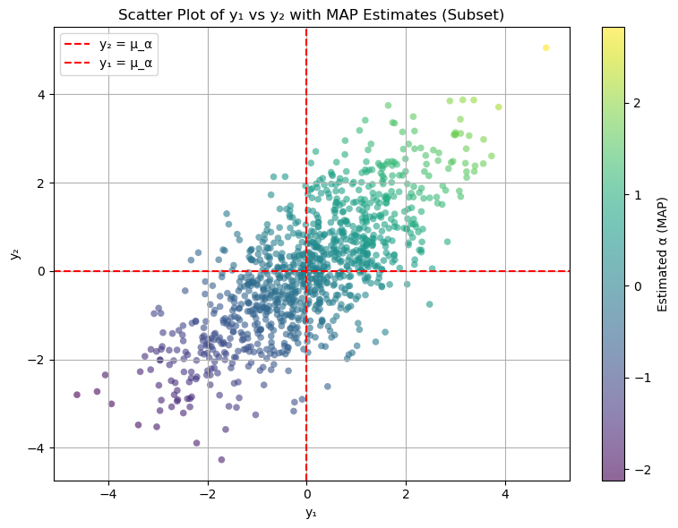
# Scatter plot of y1 vs y2 with color representing alpha_map
plt.figure(figsize=(8, 6))
scatter = plt.scatter(
    y1_subset,
    y2_subset,
    c=alpha_estimates_subset,
    cmap='viridis',
    alpha=0.6,
    marker='o',
    edgecolor='none',
    s=30
)
plt.colorbar(scatter, label='Estimated α (MAP)')
plt.axhline(mu_alpha, color='red', linestyle='--', linewidth=1.5, label='y₂ = μ_α')
plt.axvline(mu_alpha, color='red', linestyle='--', linewidth=1.5, label='y₁ = μ_α')
plt.title('Scatter Plot of y₁ vs y₂ with MAP Estimates (Subset)')
plt.xlabel('y₁')
plt.ylabel('y₂')
plt.legend()
plt.grid(True)
plt.tight_layout()
plt.show()
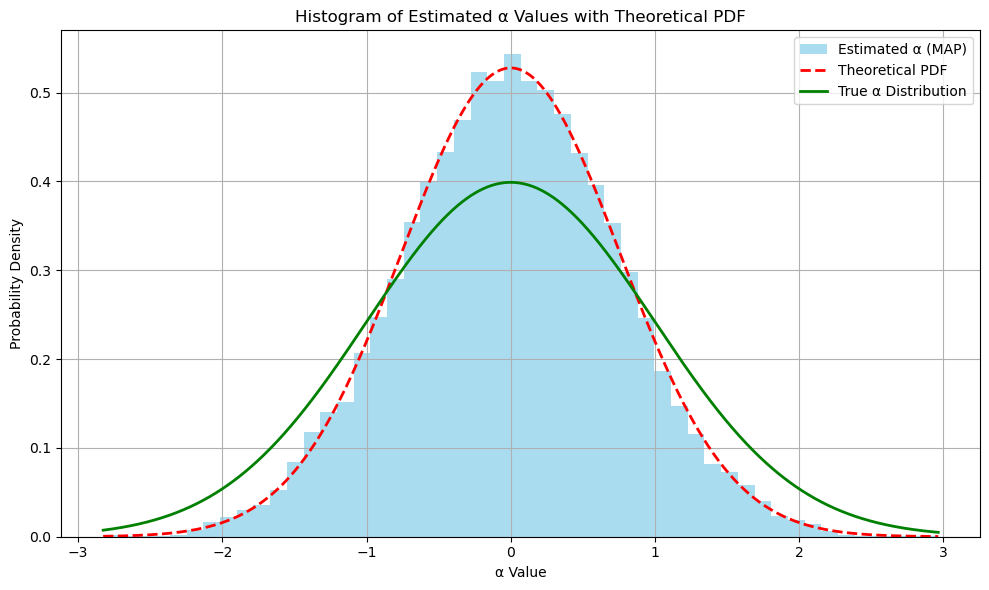
Simulation Results with Random α_true:
Prior Mean (mu_alpha): 0
MAP Estimator Mean: -0.0042
Theoretical Expected Mean: 0.0000
Bias: -0.0042
MAP Estimator Std Dev: 0.7542
Theoretical Std Dev: 0.7559

# Visualization

# Define the number of points to plot for the subset
subset_size = 100  # Number of points to include in the subset scatter plot

# Select the first 'subset_size' simulation runs
subset_indices = np.arange(1, subset_size + 1)
subset_est_alpha = alpha_estimates[:subset_size]
subset_true_alpha = alpha_true[:subset_size]  # Correctly extract the true alpha values

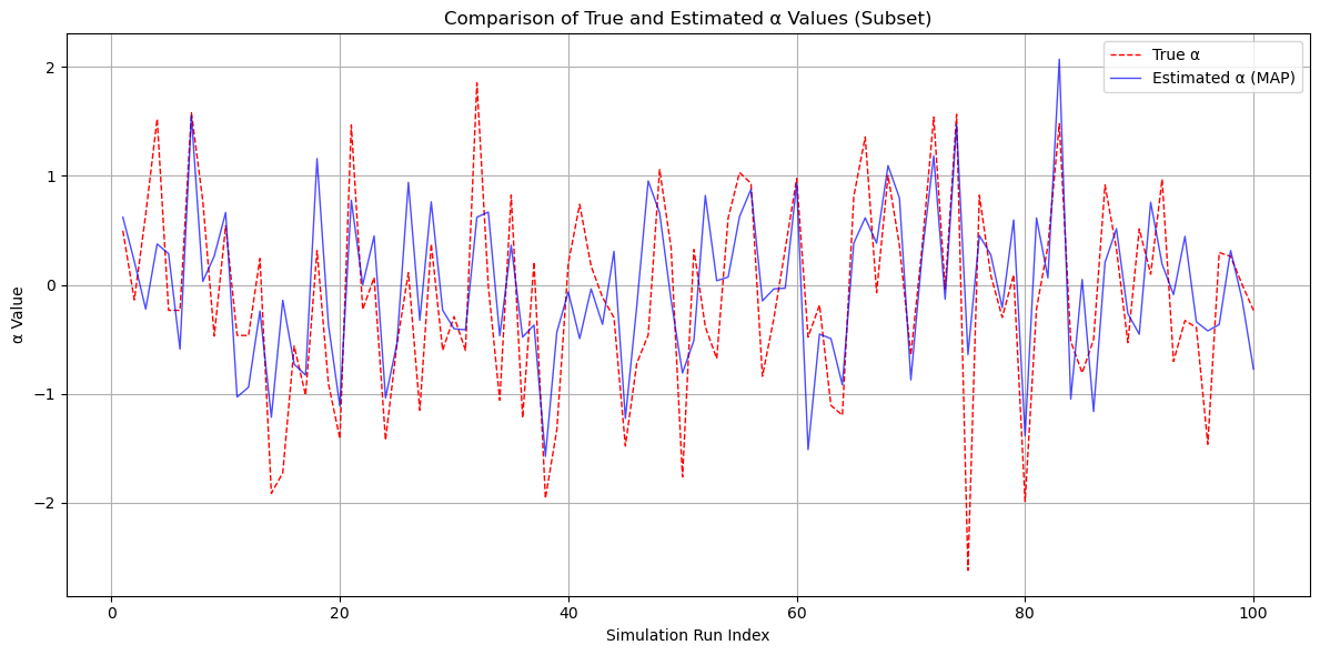
# Plotting the comparison
plt.figure(figsize=(12, 6))

plt.plot(subset_indices, subset_true_alpha, label='True α', color='red', linestyle='--', linewidth=1)
plt.plot(subset_indices, subset_est_alpha, label='Estimated α (MAP)', color='blue', alpha=0.7, linewidth=1)

plt.title('Comparison of True and Estimated α Values (Subset)')
plt.xlabel('Simulation Run Index')
plt.ylabel('α Value')
plt.legend()
plt.grid(True)
plt.tight_layout()
plt.show()

from scipy.stats import norm

# Plotting the histogram of estimated alphas
plt.figure(figsize=(10, 6))

# Histogram of alpha_estimates
count, bins, patches = plt.hist(
    alpha_estimates,
    bins=50,
    alpha=0.7,
    label='Estimated α (MAP)',
    color='skyblue',
    density=True  # Normalize the histogram to form a probability density
)

# Overlay the theoretical PDF of the MAP estimator
# The theoretical distribution of alpha_estimates is Gaussian with:
# Mean: theoretical_mean
# Standard Deviation: theoretical_std
# From previous calculations:
# theoretical_mean = 0 (since mu_alpha = 0)
# theoretical_std = sqrt((sigma_alpha2 / denominator)^2 * (4 * sigma_alpha2 + 2 * sigma2 * (1 + rho)))
theoretical_mean = 0  # As per prior calculations
theoretical_std = np.sqrt((sigma_alpha2 / denominator) ** 2 * (4 * sigma_alpha2 + 2 * sigma2 * (1 + rho)))

# Generate points for the theoretical PDF
x = np.linspace(min(alpha_estimates), max(alpha_estimates), 1000)
pdf = norm.pdf(x, loc=theoretical_mean, scale=theoretical_std)

# Plot the theoretical PDF
plt.plot(x, pdf, 'r--', linewidth=2, label='Theoretical PDF')

# Plot the true alpha distribution
# Since alpha_true is sampled from N(mu_alpha, sigma_alpha2), overlay its PDF
true_pdf = norm.pdf(x, loc=mu_alpha, scale=np.sqrt(sigma_alpha2))
plt.plot(x, true_pdf, 'g-', linewidth=2, label='True α Distribution')

plt.title('Histogram of Estimated α Values with Theoretical PDF')
plt.xlabel('α Value')
plt.ylabel('Probability Density')
plt.legend()
plt.grid(True)
plt.tight_layout()
plt.show()

