Matched Filter

The correlation receiver implementations discussed earlier rely on computing integrals of the form:

\[ r_x = \int_{-\infty}^{\infty} r(t) x(t) \, dt \]

where \( r(t) \) is the received signal, and \( x(t) \) is either a basis function \( \phi_j(t) \) (in the first version) or a signal waveform \( s_m(t) \) (in the second version). This operation extracts the component of \( r(t) \) aligned with \( x(t) \), forming the basis for the MAP decision rule. An alternative approach that achieves the same result is the matched filter, a filtering technique that maximizes the output signal-to-noise ratio.

The matched filter has an impulse response given by:

\[ h(t) = x(T - t), \]

where \( T \) is an arbitrary time instant, typically chosen to match the signal duration or a convenient sampling point. This impulse response is a time-reversed version of \( x(t) \), effectively flipping it around \( t = T/2 \) if \( T \) is the endpoint of the signal.

When \( r(t) \) is passed through this filter, the output is given by the convolution:

\[ y(t) = r(t) \circledast h(t) = \int_{-\infty}^{\infty} r(\tau) h(t - \tau) \, d\tau. \]

Substituting \( h(t) = x(T - t) \), the convolution simplifies to:

\[ y(t) = \int_{-\infty}^{\infty} r(\tau) x(T - t + \tau) \, d\tau. \]

Evaluating at \( t = T \), we obtain:

\[ y(T) = \int_{-\infty}^{\infty} r(\tau) x(T - T + \tau) \, d\tau = \int_{-\infty}^{\infty} r(\tau) x(\tau) \, d\tau = r_x. \]

Thus, the filter output at \( t = T \) exactly equals the correlation \( r_x \). Instead of explicitly computing the integral as in the correlation receiver, the matched filter allows the receiver to pass \( r(t) \) through a filter matched to \( x(t) \) and sample the output at time \( T \) to obtain the same result. This approach provides a continuous-time alternative to the discrete correlation operation, with the sampling time \( T \) chosen to align with the signal’s duration or a point of maximum signal energy.

The term “matched” reflects the fact that \( h(t) \) is specifically designed to maximize the response to \( x(t) \), enhancing the desired signal component while suppressing noise. This equivalence makes the matched filter a powerful tool for implementing optimal receivers, particularly in hardware, where filtering operations are naturally suited for real-time signal processing.

Matched Filter Receiver Structure

The matched filter approach can replace the correlators in either version of the correlation receiver, providing an alternative yet mathematically equivalent method for implementing the MAP decision rule.

First Version: Basis Function Matching

This version uses \( N \) matched filters, each with an impulse response:

\[ h_j(t) = \phi_j(T - t). \]

Each matched filter outputs:

\[ r_j = \int_{-\infty}^{\infty} r(t) \phi_j(t) \, dt, \]

which is obtained at the sampling instant \( t = T \) as \( y_j(T) \). The receiver then forms the vector:

\[ \vec{r} = [r_1, r_2, \ldots, r_N], \]

and computes the decision metric for each possible transmitted signal:

\[ \vec{r} \cdot \vec{s}_m + \eta_m. \]

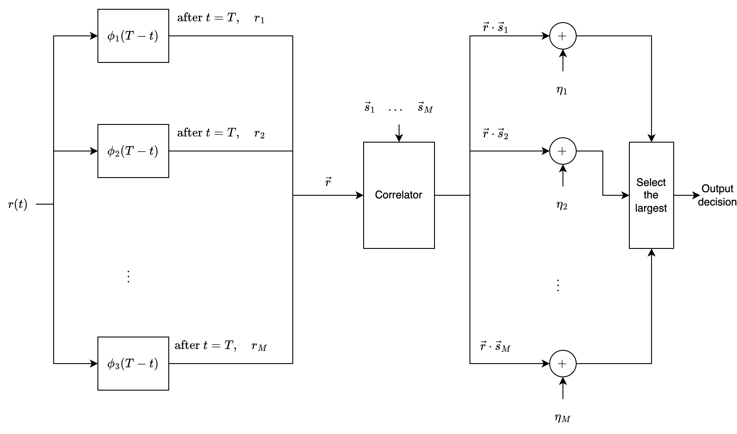Illustration of a matched filter receiver with \(N\) correlators.

Second Version: Signal Matching

This version uses \( M \) matched filters, each with an impulse response:

\[ h_m(t) = s_m(T - t). \]

Each matched filter outputs:

\[ \int_{-\infty}^{\infty} r(t) s_m(t) \, dt, \]

which is obtained at \( t = T \) as \( y_m(T) \). The receiver then adds the bias term \( \eta_m \) and selects the signal with the maximum metric.

Structural Comparison

• Basis Function Matching (First Version): Uses \( N \) parallel matched filters for the basis functions, followed by a vector operation to compute the final decision metric.

• Signal Matching (Second Version): Uses \( M \) parallel matched filters, each directly matched to a signal waveform, producing decision metrics without requiring a separate vector computation.

Implementation Considerations

Both structures achieve the MAP rule, differing only in where the filtering is applied.

• If the system is already structured around basis functions, the first version is natural.

• If the system directly works with waveform templates, the second version simplifies implementation.

Both implementations are widely used in practical communication systems, where filtering operations align well with hardware-based signal processing.

Example: Matched Filter for Biorthogonal Signaling

Consider a biorthogonal signaling system with \( M = 4 \) signals, constructed from two orthogonal signals. These signals are used to transmit information over an AWGN channel with noise power spectral density \( N_0/2 \).

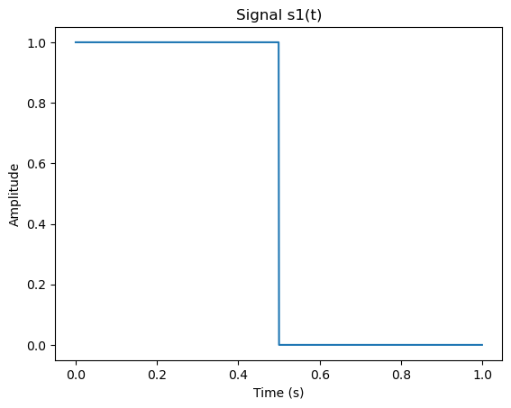
The signals consist of two orthogonal waveforms, \( s_1(t) \) and \( s_3(t) \), with their negations forming the biorthogonal set:

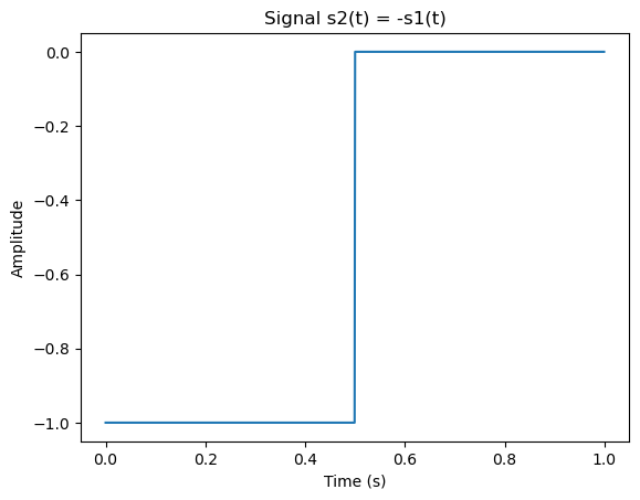
• \( s_2(t) = -s_1(t) \)

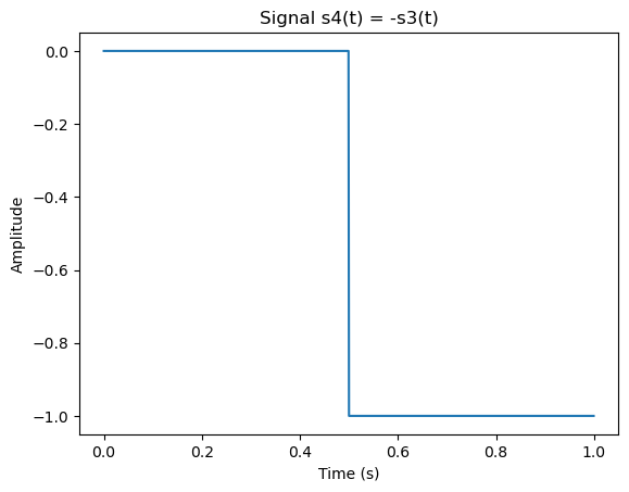
• \( s_4(t) = -s_3(t) \)

Assume the waveforms are rectangular pulses:

• \( s_1(t) = A \) for \( 0 \leq t \leq T/2 \), and zero elsewhere.

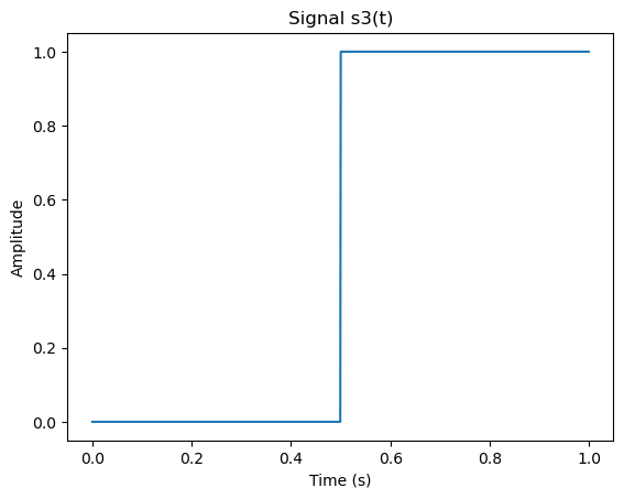
• \( s_3(t) = A \) for \( T/2 < t \leq T \), and zero elsewhere.

• \( A \) is the amplitude, and \( T \) is the signal duration.

Step 1: Determine Basis Functions

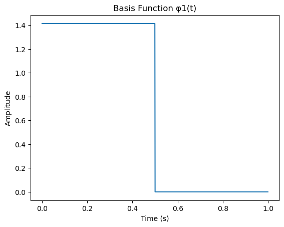
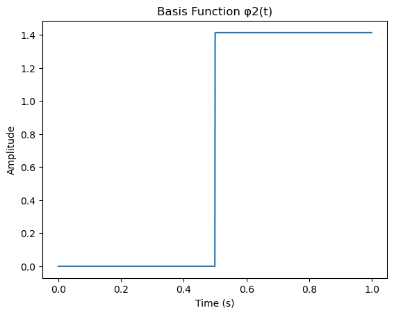
Since the signals span a 2D signal space (\( N = 2 \)), we define two orthonormal basis functions:

\[\begin{split} \phi_1(t) = \begin{cases} \sqrt{\frac{2}{T}}, & 0 \leq t \leq \frac{T}{2} \\ 0, & \text{otherwise} \end{cases} \end{split}\]

\[\begin{split} \phi_2(t) = \begin{cases} \sqrt{\frac{2}{T}}, & \frac{T}{2} < t \leq T \\ 0, & \text{otherwise} \end{cases} \end{split}\]

The orthonormality is verified:

\[ \int_0^{T/2} \phi_1^2(t) \, dt = \frac{2}{T} \times \frac{T}{2} = 1, \quad \int_{T/2}^{T} \phi_2^2(t) \, dt = \frac{2}{T} \times \frac{T}{2} = 1. \]

Since their supports do not overlap, they are also orthogonal:

\[ \int_{-\infty}^{\infty} \phi_1(t) \phi_2(t) \, dt = 0. \]

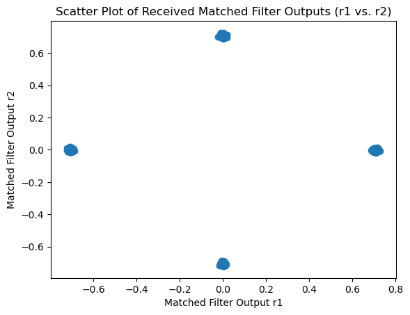
The signal representations in this basis are:

• \( s_1(t) = A \phi_1(t) \), so \( \vec{s}_1 = (\sqrt{E}, 0) \)

• \( s_2(t) = -s_1(t) \), so \( \vec{s}_2 = (-\sqrt{E}, 0) \)

• \( s_3(t) = A \phi_2(t) \), so \( \vec{s}_3 = (0, \sqrt{E}) \)

• \( s_4(t) = -s_3(t) \), so \( \vec{s}_4 = (0, -\sqrt{E}) \)

where \( E = \frac{1}{2} A^2 T \) is the signal energy.

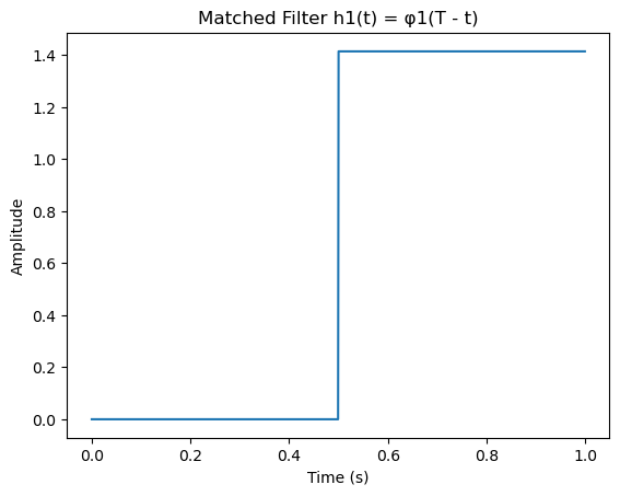
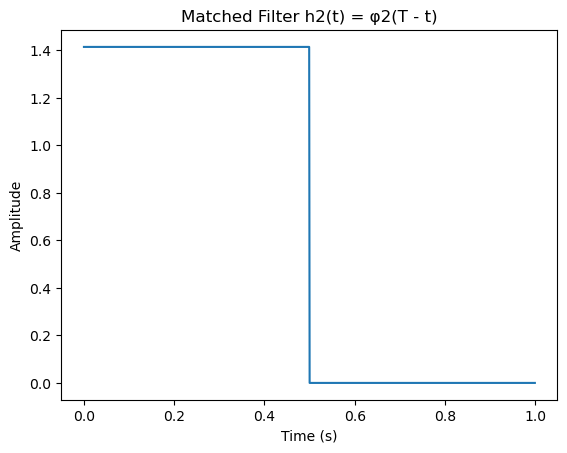
Step 2: Matched Filter Impulse Responses

The matched filters for the basis functions have impulse responses:

\[\begin{split} h_1(t) = \phi_1(T - t) = \begin{cases} \sqrt{\frac{2}{T}}, & \frac{T}{2} \leq t \leq T \\ 0, & \text{otherwise} \end{cases} \end{split}\]

\[\begin{split} h_2(t) = \phi_2(T - t) = \begin{cases} \sqrt{\frac{2}{T}}, & 0 \leq t \leq \frac{T}{2} \\ 0, & \text{otherwise} \end{cases} \end{split}\]

These are time-reversed versions of \( \phi_1(t) \) and \( \phi_2(t) \), ensuring that the peak correlation occurs at \( t = T \).

Step 3: Noise-Free Matched Filter Responses

If \( s_1(t) \) is transmitted, the received signal is:

\[ r(t) = s_1(t) + n(t), \]

where \( s_1(t) = A \) for \( 0 \leq t \leq T/2 \), and zero elsewhere.

Applying the matched filters:

\[ y_1(t) = \int_{-\infty}^{\infty} s_1(\tau) h_1(t - \tau) \, d\tau. \]

For \( t = T/2 \), partial overlap exists. At \( t = T \), the overlap is complete:

\[ y_1(T) = \int_0^{T/2} A \sqrt{\frac{2}{T}} \, d\tau = A \sqrt{\frac{T}{2}} = \sqrt{E}. \]

For the second filter:

\[ y_2(t) = \int_{-\infty}^{\infty} s_1(\tau) h_2(t - \tau) \, d\tau. \]

Since \( s_1(t) \) and \( h_2(t) \) do not overlap, we get:

\[ y_2(T) = 0. \]

Thus, the matched filter outputs for \( s_1(t) \) are:

\[ y_{1s}(T) = \sqrt{E}, \quad y_{2s}(T) = 0. \]

Step 4: Received Vector with Noise

Including noise, the received vector is:

\[ \vec{r} = (r_1, r_2) = (\sqrt{E} + n_1, n_2), \]

where the noise components are:

\[ n_k = y_{kn}(T) = \int_0^T n(t) \phi_k(t) \, dt. \]

Since \( n(t) \) is AWGN, the noise projections \( n_k \sim \mathcal{N}(0, N_0/2) \) due to the basis functions’ normalization.

import numpy as np
import matplotlib.pyplot as plt

# 1) Parameters
T = 1.0
A = 1.0
Ns = 1000
dt = T / Ns
time = np.arange(0, T, dt)
half_index = Ns // 2
EbN0_dB = 10

# Derived energy and noise
E = 0.5 * A**2 * T  # for these biorthogonal signals
EbN0_lin = 10**(EbN0_dB/10.0)
N0 = 2 * E / EbN0_lin
noise_var = N0 / 2.0

# 2) Define signals s1, s2, s3, s4
s1 = np.zeros_like(time); s1[:half_index] = A
s2 = -s1
s3 = np.zeros_like(time); s3[half_index:] = A
s4 = -s3

# Plot them
plt.figure()
plt.plot(time, s1)
plt.title("Signal s1(t)")
plt.xlabel("Time (s)")
plt.ylabel("Amplitude")
plt.show()

plt.figure()
plt.plot(time, s2)
plt.title("Signal s2(t) = -s1(t)")
plt.xlabel("Time (s)")
plt.ylabel("Amplitude")
plt.show()

plt.figure()
plt.plot(time, s3)
plt.title("Signal s3(t)")
plt.xlabel("Time (s)")
plt.ylabel("Amplitude")
plt.show()

plt.figure()
plt.plot(time, s4)
plt.title("Signal s4(t) = -s3(t)")
plt.xlabel("Time (s)")
plt.ylabel("Amplitude")
plt.show()

# 3) Define basis functions phi1, phi2
phi1 = np.zeros_like(time); phi1[:half_index] = np.sqrt(2.0 / T)
phi2 = np.zeros_like(time); phi2[half_index:] = np.sqrt(2.0 / T)

# Plot basis functions
plt.figure()
plt.plot(time, phi1)
plt.title("Basis Function φ1(t)")
plt.xlabel("Time (s)")
plt.ylabel("Amplitude")
plt.show()

plt.figure()
plt.plot(time, phi2)
plt.title("Basis Function φ2(t)")
plt.xlabel("Time (s)")
plt.ylabel("Amplitude")
plt.show()

# 4) Matched filters h1, h2 (reversed phi1, phi2)
h1 = phi1[::-1]
h2 = phi2[::-1]

# Plot matched filters
plt.figure()
plt.plot(time, h1)
plt.title("Matched Filter h1(t) = φ1(T - t)")
plt.xlabel("Time (s)")
plt.ylabel("Amplitude")
plt.show()

plt.figure()
plt.plot(time, h2)
plt.title("Matched Filter h2(t) = φ2(T - t)")
plt.xlabel("Time (s)")
plt.ylabel("Amplitude")
plt.show()

# 5) Noise-free demonstration: convolve s1 with h1, h2
y1_s1 = np.convolve(s1, h1, mode='full') * dt
y2_s1 = np.convolve(s1, h2, mode='full') * dt
sample_index = Ns - 1  # index corresponding to t=T
print("Noise-free outputs for s1(t):")
print(f"y1(T) = {y1_s1[sample_index]:.3f}  (theory ~ sqrt(E) = {np.sqrt(E):.3f})")
print(f"y2(T) = {y2_s1[sample_index]:.3f}  (theory = 0)")

# 6) Full random symbol transmission
signals = [s1, s2, s3, s4]
ideal_vectors = np.array([
    [ np.sqrt(E),  0.0       ], 
    [-np.sqrt(E),  0.0       ], 
    [ 0.0,         np.sqrt(E)], 
    [ 0.0,        -np.sqrt(E)]
])
num_symbols = 2000
tx_symbols = np.random.randint(0, 4, size=num_symbols)
r1_vals = np.zeros(num_symbols)
r2_vals = np.zeros(num_symbols)

for i in range(num_symbols):
    s_tx = signals[ tx_symbols[i] ]
    noise = np.random.normal(0, np.sqrt(noise_var), size=Ns)
    r = s_tx + noise
    
    y1 = np.convolve(r, h1, mode='full') * dt
    y2 = np.convolve(r, h2, mode='full') * dt
    
    r1_vals[i] = y1[sample_index]
    r2_vals[i] = y2[sample_index]

# Decision
decisions = np.zeros(num_symbols, dtype=int)
for i in range(num_symbols):
    r_vec = np.array([r1_vals[i], r2_vals[i]])
    distances = np.sum((r_vec - ideal_vectors)**2, axis=1)
    decisions[i] = np.argmin(distances)

errors = np.sum(decisions != tx_symbols)
SER = errors / num_symbols
print(f"Symbol Error Rate (SER) at Eb/N0 = {EbN0_dB} dB is {SER:.4f}")

# 7) Scatter plot of matched filter outputs
subset = 500
plt.figure()
plt.scatter(r1_vals[:subset], r2_vals[:subset], marker='o')
plt.title("Scatter Plot of Received Matched Filter Outputs (r1 vs. r2)")
plt.xlabel("Matched Filter Output r1")
plt.ylabel("Matched Filter Output r2")
plt.show()

Noise-free outputs for s1(t):
y1(T) = 0.707  (theory ~ sqrt(E) = 0.707)
y2(T) = 0.000  (theory = 0)
Symbol Error Rate (SER) at Eb/N0 = 10 dB is 0.0000