MiniMax Criterion#
MOTIVATION. The question is what issues of the Bayes and MAP criteria lead to the need for a new criterion?
The Bayes criterion requires both costs and a priori probabilities to set the threshold.
The MAP criterion needs only the a priori probabilities; it does not require knowledge of the costs.
In contradistinction, the minimax criterion does require knowledge of the costs but does not use the a priori probabilities.
Bayes risk review#
We use the setting in the antipodal signal dection example.
Previous problem setting with given fixed prior probabilities \(\pi_0\) and \(\pi_1\).
import warnings
warnings.filterwarnings("ignore")
from scipy.special import erf, erfc
import numpy as np
import matplotlib.pyplot as plt

# Given parameters
b = 1  # s1 = b, s0 = -b
sigma_squared = 0.25
sigma = np.sqrt(sigma_squared)
pi_0_fixed = 0.8  # given fixed prior probability for H0
pi_1_fixed = 0.2  # given fixed prior probability for H1

# Costs
C00 = 0  # Correct decision, H0
C11 = 0  # Correct decision, H1
C10 = 1  # Incorrect decision, H1|H0
C01 = 2  # Incorrect decision, H0|H1

# Calculate tau'
tau_map_fixed = pi_0_fixed / pi_1_fixed
tau_prime_fixed = (sigma_squared / (2 * b)) * np.log(tau_map_fixed)

# Define Pij based on the problem's conditions
def P00(tau_prime):
    return 0.5 * (1 + erf((tau_prime + b) / (sigma * np.sqrt(2))))

def P01(tau_prime):
    return 0.5 * (1 + erf((tau_prime - b) / (sigma * np.sqrt(2))))

def P10(tau_prime):
    return 0.5 * erfc((tau_prime + b) / (sigma * np.sqrt(2)))

def P11(tau_prime):
    return 0.5 * erfc((tau_prime - b) / (sigma * np.sqrt(2)))
Bayes risk as a function of \(\pi_0\)#
Then the Bayes risk (average risk) \( r \) is
The Bayes risk at \( \pi_0 = a \), where \(a\) is a specific value of \(\pi_0\), is shown in the following figure.
# The decision threshold tau_B is derived from the Bayes criterion
def bayes_risk(pi_0):
    pi_1 = 1 - pi_0
    tau_B = (pi_0 * (C10 - C00)) / (pi_1 * (C01 - C11))
    tau_prime_B = (sigma_squared / (2 * b)) * np.log(tau_B)
    # Calculate Pij values for the current pi_0
    P00_val = P00(tau_prime_B)
    P01_val = P01(tau_prime_B)
    P10_val = P10(tau_prime_B)
    P11_val = P11(tau_prime_B)
    # Calculate r0(a) and r1(a)
    r0_B = C10 * P10_val + C00 * P00_val
    r1_B = C01 * P01_val + C11 * P11_val
    # Calculate the Bayes risk
    return pi_0 * r0_B + pi_1 * r1_B

# Define the range of pi0 and the value of 'a'
pi0_values = np.linspace(0, 1, 500)
a = 0.6  # Specific value of pi_0 for the stem plot

# Calculate Bayes risk for each value of pi_0
bayes_r_values = [bayes_risk(pi_0) for pi_0 in pi0_values]
bayes_r_at_a = bayes_risk(a)

# Plotting the Bayes risk function
plt.figure(figsize=(6, 4))
plt.plot(pi0_values, bayes_r_values, label='Bayes Risk $r(\pi_0)$', color='blue')

# Add the stem plot for the specific value a
plt.stem([a], [bayes_r_at_a], linefmt='r-', markerfmt='ro', basefmt=" ")

# Annotate the point a
plt.text(a, bayes_r_at_a, f'($\pi_0 = {a}$, $r(a) = {bayes_r_at_a:.2f}$)', fontsize=12, color='red')

# Define the constants again for the boundaries
C_00_value = C00 # previously defined as 0
C_11_value = C11 # previously defined as 0

# Calculate Bayes risk values at pi0 = 0 and pi0 = 1
pi0_0_r = C_11_value
pi0_1_r = C_00_value

# Add the points for pi0 = 0 and pi0 = 1
plt.plot(0, pi0_0_r, 'go')  # Point at pi0 = 0, r = C_11
plt.text(0, pi0_0_r, '$C_{11}$', fontsize=12, color='green')

plt.plot(1, pi0_1_r, 'go')  # Point at pi0 = 1, r = C_00
plt.text(1, pi0_1_r, '$C_{00}$', fontsize=12, color='green')

# Plot settings
plt.title('Bayes Risk $r(\pi_0)$ as a Function of $\\pi_0$ with Highlighted Value at $a$', fontsize=16)
plt.xlabel('$\pi_0$', fontsize=14)
plt.ylabel('Bayes Risk $r$', fontsize=14)
plt.grid(True)
plt.legend()
plt.show()
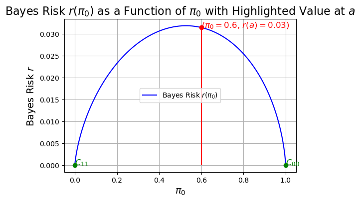
In most cases, \( r \) is larger at intermediate values of \( \pi_0 \).
Indeed, it is straightforward to show that \( r \) is a concave function in \( \pi_0 \).
DISCUSSION. To illustrate the need for the minimax criterion, consider an example of the Bayes risk \( r \) as a function of the a priori probability \( \pi_0 \)
Assuming \( \pi_0 = 0 \).
Recall that the variable \( \pi_0 \) represents the prior probability of hypothesis \( H_0 \) being true.
If \( \pi_0 = 0 \), this means that we are certain that \( H_0 \) is false, and thus, \( H_1 \) is true.
Consequently, we have the complementary probability \( \pi_1 = 1 \), since \( \pi_1 = 1 - \pi_0 \).
Bayes risk for \( \pi_0 = 0 \):
The Bayes risk is given by the general formula:
since \( \pi_0 = 0 \)
Since \( \pi_1 = 1 \), the equation simplifies further:
Additionally, for the assumption of \(\pi_0=0\), we have that:
\( P_{01} = 0 \), which means there is no chance of making an error by deciding \( D_0 \) when \( H_1 \) is true.
\( P_{11} = 1 \), which means we always decide \( D_1 \) when \( H_1 \) is true.
Substituting these values into the equation, we have
Thus, assuming \(\pi_0=0\), when \( H_1 \) is true and we decide \( D_1 \) (correctly), the Bayes risk equals \( C_{11} \), the cost of making that decision.
This means the decision incurs the cost \( C_{11} \), even though it’s correct, reflecting the inherent cost of acting on the decision.
On the other hand, if \( \pi_0 = 1 \), a similar argument shows that \( r = C_{00} \).
This example leads to the need for minimax because it highlights how the Bayes risk depends on prior probabilities, which may not always be known or reliable.
The minimax criterion provides a way to safeguard against the worst-case scenario, ensuring that the decision-maker minimizes the maximum potential loss, regardless of the true value of \( \pi_0 \) or \( \pi_1 \).
Actual risk#
Actual risk is defined when the a priori probability is unknown and guessed.
Assume that we guess the a priori probability is some specific value \( \pi_0 = a \).
This returns a specific decision rule \( \delta_B \) with a specific Bayes threshold, set at
For a given guess of the prior probability \(\pi_0\), the actual risk \( r(\pi_0, a) \) for that guess is obtained as
where \( r_0(a) \) and \( r_1(a) \) are conditional risks for each hypothesis when the threshold and decision rule are controlled by \( a \).
The conditional risk is defined as
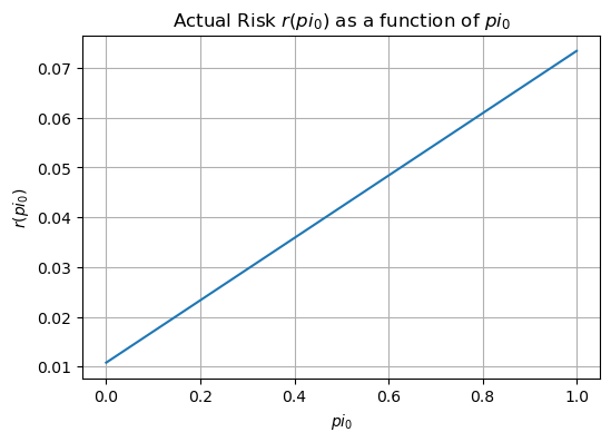
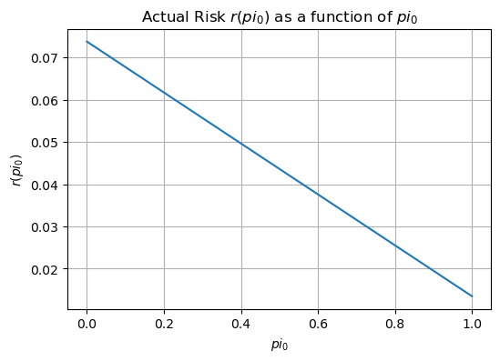
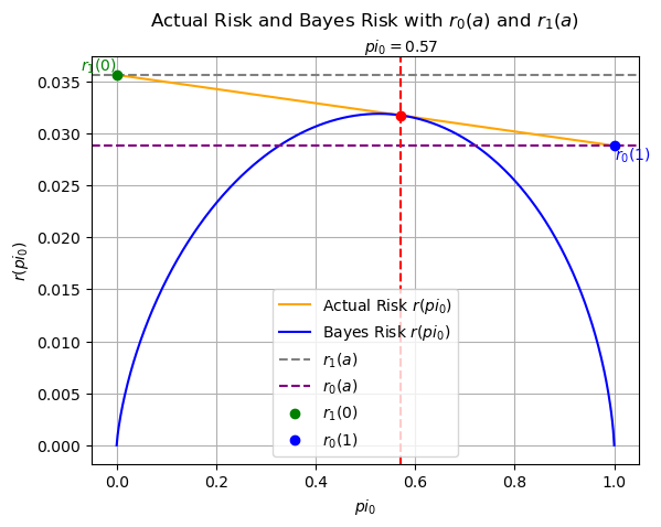
Since \( r_0(a) \) and \( r_1(a) \) are constants for a specific value of \( a \), the actual risk is linear in \( \pi_0 \).
If our guess of \( \pi_0 = a \) is correct, the actual risk is identical to the Bayes risk.
On the other hand, if \( \pi_0 = 1 \) were the “true” value, the actual risk we would entail in this example would be \( r_0(a) \).
Actual risk as a function of \(\pi_0\)#
# Define the actual risk function r(pi0, a)
def actual_risk(pi_0,a):

    pi_0_fixed = a  # given fixed prior probability for H0
    pi_1_fixed = 1 - a  # given fixed prior probability for H1
    # Calculate tau'
    tau_map_fixed = pi_0_fixed / pi_1_fixed
    tau_prime_fixed = (sigma_squared / (2 * b)) * np.log(tau_map_fixed)
    pi_1 = 1 - pi_0
    # Calculate Pij values for the current pi_0
    P00_val = P00(tau_prime_fixed)
    P01_val = P01(tau_prime_fixed)
    P10_val = P10(tau_prime_fixed)
    P11_val = P11(tau_prime_fixed)
    # Calculate r0(a) and r1(a)
    r0 = C10 * P10_val + C00 * P00_val
    r1 = C01 * P01_val + C11 * P11_val
    # Calculate the actual risk
    return pi_0 * r0 + pi_1 * r1

a = 0.1  # we guess that the prior probability of H0 is 0.1
r_values = [actual_risk(pi_0,a) for pi_0 in pi0_values]

# Plotting the actual risk as a function of pi0
plt.figure(figsize=(6, 4))
plt.plot(pi0_values, r_values, label='$r(pi_0)$')
plt.title('Actual Risk $r(pi_0)$ as a function of $pi_0$')
plt.xlabel('$pi_0$')
plt.ylabel('$r(pi_0)$')
plt.grid(True)
plt.show()
a = 0.7  # we guess that the prior probability of H0 is 0.7
r_values = [actual_risk(pi_0,a) for pi_0 in pi0_values]

# Plotting the actual risk as a function of pi0
plt.figure(figsize=(6, 4))
plt.plot(pi0_values, r_values, label='$r(pi_0)$')
plt.title('Actual Risk $r(pi_0)$ as a function of $pi_0$')
plt.xlabel('$pi_0$')
plt.ylabel('$r(pi_0)$')
plt.grid(True)
plt.show()
Actual and Bayes risks as a function of \(\pi_0\)#
# Recalculate r1(a) and r0(a) with a specific value of `a`
a = 0.4
sigma_squared = 0.25
b = 1
pi_0_fixed = a  # given fixed prior probability for H0
pi_1_fixed = 1 - a  # given fixed prior probability for H1

# Calculate tau'
tau_map_fixed = pi_0_fixed / pi_1_fixed
tau_prime_fixed = (sigma_squared / (2 * b)) * np.log(tau_map_fixed)
r1_a = C01 * P01(tau_prime_fixed) + C11 * P11(tau_prime_fixed)
r0_a = C10 * P10(tau_prime_fixed) + C00 * P00(tau_prime_fixed)

r_values = [actual_risk(pi_0,a) for pi_0 in pi0_values]

# Find the intersection point between actual risk and Bayes risk
diff = np.abs(np.array(r_values) - np.array(bayes_r_values))
intersection_index = np.argmin(diff)
intersection_pi0 = pi0_values[intersection_index]
intersection_risk = r_values[intersection_index]

# Calculate the endpoints of the actual risk
r1_0 = r_values[0]  # Actual risk at pi_0 = 0
r0_1 = r_values[-1]  # Actual risk at pi_0 = 1
# index -1 means the last value in the array

# Create a plot with additional annotations
plt.figure(figsize=(6, 4))
fig, ax = plt.subplots()

# Plotting the actual risk and Bayes risk
ax.plot(pi0_values, r_values, label='Actual Risk $r(pi_0)$', color='orange')
ax.plot(pi0_values, bayes_r_values, label='Bayes Risk $r(pi_0)$', color='blue')

# Annotating r1(a) and r0(a)
ax.axhline(y=r1_a, color='gray', linestyle='--', label='$r_1(a)$')
ax.axhline(y=r0_a, color='purple', linestyle='--', label='$r_0(a)$')

# Annotating the intersection point
ax.plot(intersection_pi0, intersection_risk, 'ro')  # Point
ax.axvline(intersection_pi0, color='red', linestyle='--')  # Projection on x-axis
ax.text(intersection_pi0, ax.get_ylim()[1], f'$pi_0 = {intersection_pi0:.2f}$', ha='center', va='bottom')

# Annotating the endpoints r1(0) and r0(1)
ax.plot(0, r1_0, 'go', label='$r_1(0)$')  # Endpoint r1(0)
ax.plot(1, r0_1, 'bo', label='$r_0(1)$')  # Endpoint r0(1)

# Adding labels for endpoints
ax.text(0, r1_0, f'$r_1(0)$', ha='right', va='bottom', color='green')
ax.text(1, r0_1, f'$r_0(1)$', ha='left', va='top', color='blue')

# Setting labels and title
ax.set_title('Actual Risk and Bayes Risk with $r_0(a)$ and $r_1(a)$ \n')
ax.set_xlabel('$pi_0$')
ax.set_ylabel('$r(pi_0)$')

# Adding grid, legend, and show plot
ax.grid(True)
ax.legend()
plt.show()
<Figure size 600x400 with 0 Axes>
Decision using MiniMax Criterion#
OBJECTIVE. The minimax criterion minimizes the maximum risk.
The maximin criterion also maximizes the minimum risk.
In the example above, the minimax criterion would assume the value of \( \pi_0 \) such that the actual risk is a constant represented by the dashed line.
Decision Making#
METHODOLOGY. The question is how to use the minimax criterion to make decision \(D_0\) or \(D_1\).
Three different situations must be examined in determining the minimax criterion.
The case where the minimax criterion corresponds to \( \pi_0 = 0 \) or \( \pi_0 = 1 \).
The case where the minimax solution corresponds to \( \pi_0 \) interior to the interval \( (0, 1) \) and the Bayes risk is differentiable at this solution.
The case where the minimax solution corresponds to \( \pi_0 \) interior to \( (0, 1) \) but the Bayes risk is not differentiable at this solution.
Each of these cases is presented in one of the following sections.
Endpoint Minimax Solution#
In some cases of using the Bayes risk, the minimax solution is to always decide \( D_1 \).
Since the minimax risk for an endpoint maximum is always either \( C_{00} \) or \( C_{11} \), the easiest way to determine this case is to first try to find a minimax solution using the approaches of the following two sections.
If this attempt is successful, we simply compare the risk so obtained with \( C_{00} \) and \( C_{11} \) and pick the maximum.
If, however, we are unsuccessful in finding an internal minimax using the approaches of the next two sections, then the minimax solution is one of the endpoints.
In this case, the risk is the maximum of \( C_{00} \) or \( C_{11} \).”
DISCUSSION. This solution applies when the minimax risk occurs at one of the endpoints of the decision space, meaning \( \pi_0 = 0 \) or \( \pi_0 = 1 \).
Decision Rule:#
If the minimax risk corresponds to \( \pi_0 = 0 \): The decision rule would be to always choose \( H_1 \) since the risk associated with \( C_{11} \) (the cost when \( H_1 \) is true and \( H_1 \) is chosen) is considered.
Decision: Choose \( D_1 \) for any observation \( y \).
If the minimax risk corresponds to \( \pi_0 = 1 \): The decision rule would be to always choose \( H_0 \) since the risk associated with \( C_{00} \) (the cost when \( H_0 \) is true and \( H_0 \) is chosen) is considered.
Decision: Choose \( D_0 \) for any observation \( y \).
Differentiable Interior Minimax Solution#
In this case, we want to pick a value of \( \pi_0 \) such that the slope of the risk \( r(\pi_0, a) \) is zero.
From actual risk definition, differentiating \( r(\pi_0, a) \) by \( \pi_0 \), we see that the minimax solution corresponds to the point where
That is, the minimax solution corresponds to the point where the two conditional risks are identical.
We attempt to find the value of \( a \) and the associated minimax threshold \( \tau_{MM} \), given by
where \( r_0(a) = r_1(a) \).
In many practical situations, it is easier to find the decision regions \( R_0 \) and \( R_1 \) rather than the a priori probability \( a \).
This occurs when the minimax solution lies at an interior point of the decision space, typically where the conditional risks \( r_0(a) \) and \( r_1(a) \) are equal.
Decision Making Procedure#
Calculate the threshold \( \tau_{MM} \) using:
\[ \tau_{MM} = \frac{a(C_{10} - C_{00})}{(1 - a)(C_{01} - C_{11})} \]where \( a \) is the minimax a priori probability.
Calculate the likelihood ratio \( L(y) \):
\[ L(y) = \frac{p(y|H_1)}{p(y|H_0)} \]Make the decision:
If \( L(y) > \tau_{MM} \), choose \( D_1 \).
If \( L(y) \leq \tau_{MM} \), choose \( D_0 \).
Nondifferentiable Interior Minimax Solution#
This case always arises when the underlying conditional probabilities \( p(y|H_0) \) and \( p(y|H_1) \) are discrete or hybrid.
In such a case, the likelihood ratio \( L(y) \) is not differentiable everywhere.
To find the minimax solution in this case, we adopt an approach as follows.
Define two decision rules.
The first is defined by letting \( \pi_0 \) approach \( a \) from below, that is,
and it has an associated decision region for \( H_1 \) of
The second decision rule is defined by letting \( \pi_0 \) approach \( a \) from above,
Its associated decision region is
The critical region occurs when \( L(y) \) equals the threshold.
The minimax decision rule for this case of a nondifferentiable interior solution, defined around the critical region, can be stated as
and is known as a randomization rule.
If \( L(y) \) exceeds \( \tau_{MM} \), decide \( D_1 \). If \( L(y) < \tau_{MM} \), decide \( D_0 \). If \( L(y) = \tau_{MM} \), decide \( D_1 \) with probability \( \eta \).
We want to pick the variable \( \eta \) so that the conditional risk associated with decision \( D_1 \) and the decision rule \( \delta_{MM} \) is the same as the conditional risk associated with decision \( D_0 \) and \( \delta_{MM} \).
For this case, these conditional risks are labeled as \( \delta r_j \), \( j = 0, 1 \).
It is assumed that region \( R_1^- \) occurs with probability \( \eta \) and \( R_1^+ \) with probability \( (1 - \eta) \).
Now, the conditional risks are
Our guide of equality for \( j = 0 \) and \( j = 1 \) in the above equation is achieved if
DISCUSSION. This case arises when the likelihood ratio \( L(y) \) is not differentiable everywhere, often due to discrete or hybrid conditional probabilities.
Decision Making Procedure#
Define two critical values \( a^- \) and \( a^+ \):
\( a^- \) approaches \( a \) from below.
\( a^+ \) approaches \( a \) from above.
Determine the decision regions:
Region \( R_1^- \): Decision \( D_1 \) is made if \( L(y) > \frac{a^-(C_{10} - C_{00})}{(1 - a^-)(C_{01} - C_{11})} \).
Region \( R_1^+ \): Decision \( D_1 \) is made if \( L(y) > \frac{a^+(C_{10} - C_{00})}{(1 - a^+)(C_{01} - C_{11})} \).
Critical Region and Randomization:
Define a threshold \( \tau_{MM} \) around which decisions are randomized.
Decision Rule \( \delta_{MM}(y) \):
\[\begin{split} \delta_{MM}(y) = \begin{cases} 1, & L(y) > \tau_{MM} \\ \eta, & L(y) = \tau_{MM} \\ 0, & L(y) < \tau_{MM} \end{cases} \end{split}\]Here, \( \eta \) is a probability chosen such that the conditional risks are balanced.
If \( L(y) = \tau_{MM} \), the decision \( D_1 \) is made with probability \( \eta \) and \( D_0 \) with probability \( 1 - \eta \).
DISCUSSION. \( a \) represents a guessed or estimated value for the a priori probability \( \pi_0 \).
It is not necessarily the true value of \( \pi_0 \); rather, it is a value that we assume in order to set the decision threshold and determine the Bayes risk \( r(\pi_0, a) \).
The actual value of \( \pi_0 \) may differ, leading to a discrepancy between the assumed and actual risks.
The minimax criterion seeks to minimize the worst-case risk that could arise from incorrect assumptions about \( \pi_0 \).
Example: Antipodal Signal Detection and Decision Using MiniMax Criterion#
This example [B2, Ex 4.9] continues previous example, we assume that:
\( \pi_0 \) is unknown,
the costs given as previously, namely \( C_{00} = C_{11} = 0 \), \( C_{10} = 1 \), and \( C_{01} = 2 \).
Since \( C_{00} \) and \( C_{11} \) are both zero, we know that the minimax solution corresponds to an a priori probability interior to the interval \((0, 1)\); i.e., it is not an endpoint solution.
Furthermore, since this example is associated with continuous random variables, we are dealing with a differentiable interior minimax solution.
In these examples, we have used the log-likelihood ratio, and the results have shown that we decide \( D_1 \) if \( y \geq \tau_{MM}' \) and \( D_0 \) if \( y < \tau_{MM}' \), where \( \tau_{MM}' \) is the log-likelihood minimax threshold.
We want to find a threshold \( \tau_{MM}' \) such that
or, in this case,
It is easy to show that this can be written as
or
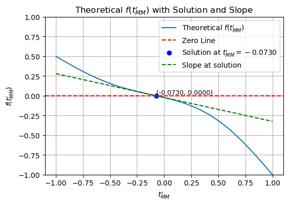
A simple way to find the solution to this transcendental equation is to define a function as
After some computation, we obtain \( \tau_{MM}' \approx -0.073 \) for \( b = 1 \) and \( \sigma^2 = 0.25 \).
Thus, the decision rule is
Numerical results#
Plot \( f \) for \( b = 1 \) and \( \sigma^2 = 0.25 \) as a function of \( \tau_{MM}' \)
# Improved version of the code including the required features
import numpy as np
import matplotlib.pyplot as plt
from scipy.special import erf
from scipy.optimize import fsolve
from scipy.misc import derivative

# Given values for the example
b = 1
sigma_squared = 0.25
sigma = np.sqrt(sigma_squared)

# Define the function f
def f(t_MM_prime):
    term1 = erf((b - t_MM_prime) / np.sqrt(2 * sigma_squared))
    term2 = 0.5 * erf((t_MM_prime + b) / np.sqrt(2 * sigma_squared))
    return term1 - term2 - 0.5

# Define the range of t_MM_prime to evaluate the function f
t_MM_prime_values = np.linspace(-1, 1, 1000)
f_values = [f(t) for t in t_MM_prime_values]

# Solve for tau_MM_prime where the function equals zero
tau_MM_prime_solution = fsolve(f, 0)[0]

# Calculate the slope at the solution point
slope_at_solution = derivative(f, tau_MM_prime_solution, dx=1e-6)

# Plot the function f and notate the solution
plt.figure(figsize=(6, 4))
plt.plot(t_MM_prime_values, f_values, label='Theoretical $f(t_{MM}^\\prime)$')
plt.axhline(0, color='red', linestyle='--', label='Zero Line')
plt.scatter(tau_MM_prime_solution, f(tau_MM_prime_solution), color='blue', label=f'Solution at $t_{{MM}}^\\prime={tau_MM_prime_solution:.4f}$')
plt.text(tau_MM_prime_solution, f(tau_MM_prime_solution), f'({tau_MM_prime_solution:.4f}, {f(tau_MM_prime_solution):.4f})', fontsize=9, verticalalignment='bottom')

# Plot the slope line at the solution
tangent_line = slope_at_solution * (t_MM_prime_values - tau_MM_prime_solution) + f(tau_MM_prime_solution)
plt.plot(t_MM_prime_values, tangent_line, color='green', linestyle='--', label='Slope at solution')

# Additional plot settings
plt.title('Theoretical $f(t_{MM}^\\prime)$ with Solution and Slope')
plt.xlabel('$t_{MM}^\\prime$')
plt.ylabel('$f(t_{MM}^\\prime)$')
plt.ylim(-1, 1)
plt.grid(True)
plt.legend()
plt.show()
import numpy as np
from scipy.special import erf
from scipy.optimize import fsolve

# Given parameters
b = 1  # Signal amplitude
sigma_squared = 0.25  # Noise variance
n_samples = 1000000  # Number of samples for simulation

# Define the function f for the Minimax criterion
def f(t_MM_prime):
    term1 = erf((b - t_MM_prime) / np.sqrt(2 * sigma_squared))
    term2 = 0.5 * erf((t_MM_prime + b) / np.sqrt(2 * sigma_squared))
    return term1 - term2 - 0.5

# Solve for the minimax threshold t_MM_prime using fsolve
t_MM_prime = fsolve(f, 0)[0]  # Initial guess is 0

# Simulate received signals and decisions based on the Minimax threshold
s0 = -b
s1 = b

# Generating noise
noise = np.random.normal(0, np.sqrt(sigma_squared), n_samples)

# Simulating received y under each hypothesis
y_given_s0 = s0 + noise
y_given_s1 = s1 + noise

# Decisions based on the Minimax threshold
decisions_s0_MM = y_given_s0 >= t_MM_prime  # Decide s1 if y >= t_MM_prime (for H0)
decisions_s1_MM = y_given_s1 >= t_MM_prime  # Decide s1 if y >= t_MM_prime (for H1)

# Estimating transmitted signals (s_hat) based on decisions for Minimax criterion
s0_hat_MM = np.where(decisions_s0_MM, s1, s0)  # Decided s1 if decision is True, else s0 (under H0)
s1_hat_MM = np.where(decisions_s1_MM, s1, s0)  # Decided s1 if decision is True, else s0 (under H1)

# Calculating empirical probabilities for Minimax criterion
P00_MM = np.mean(s0_hat_MM == s0)  # Probability of deciding H0 when H0 is true
P01_MM = np.mean(s1_hat_MM == s0)  # Probability of deciding H0 when H1 is true
P10_MM = np.mean(s0_hat_MM == s1)  # Probability of deciding H1 when H0 is true
P11_MM = np.mean(s1_hat_MM == s1)  # Probability of deciding H1 when H1 is true

# Print the results
print(f"Minimax Criterion, P00 (Decide H0 | H0 true): {P00_MM:.4f}")
print(f"Minimax Criterion, P01 (Decide H0 | H1 true): {P01_MM:.4f}")
print(f"Minimax Criterion, P10 (Decide H1 | H0 true): {P10_MM:.4f}")
print(f"Minimax Criterion, P11 (Decide H1 | H1 true): {P11_MM:.4f}")
Minimax Criterion, P00 (Decide H0 | H0 true): 0.9681
Minimax Criterion, P01 (Decide H0 | H1 true): 0.0159
Minimax Criterion, P10 (Decide H1 | H0 true): 0.0319
Minimax Criterion, P11 (Decide H1 | H1 true): 0.9841
Schonhoff’s Method#
In the following computation
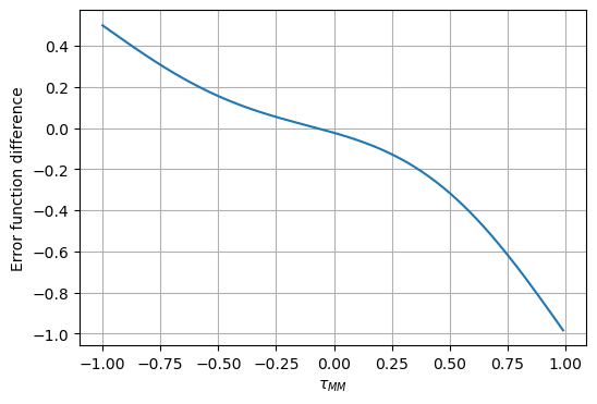
erfis used to compute the error functionfzerois used to find the zeroes of the function.efund.mandedf.mis used to find the resultedif.mis for the plot.
import numpy as np
from scipy.special import erf
from scipy.optimize import fsolve
import matplotlib.pyplot as plt

# Error function difference (EDF) function
# Inputs:
#   b = the mean for a Gaussian pdf
#   sig = standard deviation for a Gaussian pdf
#   tMM = log-likelihood minimax threshold
# Outputs:
#   Error function difference for specified tMM
def edf(tMM, b, sig):
    arg1 = (b - tMM) / (np.sqrt(2) * sig)
    arg2 = (b + tMM) / (np.sqrt(2) * sig)
    return erf(arg1) - 0.5 * erf(arg2) - 0.5

# Estimated Error Probability
# Inputs:
#   nsam = number of samples
#   snrdb = signal-to-noise ratio in dB
# Outputs:
#   Probability of error displayed for specified snr in dB
def err(nsam, snrdb):
    b = np.sqrt(12 * 10**(-0.1 * snrdb))
    n = (2 * np.random.rand(nsam) - 1) * (b / 2)
    sr = 2 * np.random.rand(nsam) - 1
    s = np.where(sr > 0, 1, -1)
    y = s + n
    d = np.where(y > 0, 1, -1)
    nerr = np.sum(d != s)
    pe = nerr / nsam
    return pe

# Error function difference solution
# Inputs:
#   b = the mean for a Gaussian pdf
#   sig = standard deviation for a Gaussian pdf
# Outputs:
#   Error function difference solution (threshold)
def efund(b, sig):
    tol = 0.01
    threshold = fsolve(lambda tMM: edf(tMM, b, sig), [-1], xtol=tol)
    return threshold[0]

# Error function difference plot
# Inputs:
#   b = the mean for a Gaussian pdf
#   sig = standard deviation for a Gaussian pdf
# Outputs:
#   Error function difference plotted versus tMM
def edif(b, sig):
    tMM = np.arange(-1, 1, 0.01)
    arg1 = (b - tMM) / (np.sqrt(2) * sig)
    arg2 = (b + tMM) / (np.sqrt(2) * sig)
    ed_plot = erf(arg1) - 0.5 * erf(arg2) - 0.5
    plt.figure(figsize=(6, 4))
    plt.plot(tMM, ed_plot)
    plt.xlabel(r'$\tau_{MM}$')
    plt.ylabel('Error function difference')
    plt.grid(True)
    plt.show()

# Example usage
if __name__ == "__main__":
    b = 1
    sig = 0.5
    nsam = 10000
    snrdb = 10

    # Estimated Error Probability
    pe = err(nsam, snrdb)
    print(f"Estimated Error Probability: {pe}")

    # Error function difference solution
    threshold = efund(b, sig)
    print(f"Minimax Threshold: {threshold}")

    # Plot Error function difference
    edif(b, sig)
Estimated Error Probability: 0.0
Minimax Threshold: -0.07301030447230179
import numpy as np
import matplotlib.pyplot as plt

# Estimated Error Probability
# Inputs:
#   nsam = number of samples
#   snrdb = signal-to-noise ratio in dB
# Outputs:
#   Probability of error displayed for specified snr in dB
def err(nsam, snrdb):
    b = np.sqrt(12 * 10**(-0.1 * snrdb))
    n = (2 * np.random.rand(nsam) - 1) * (b / 2)
    sr = 2 * np.random.rand(nsam) - 1
    s = np.where(sr > 0, 1, -1)
    y = s + n
    d = np.where(y > 0, 1, -1)
    nerr = np.sum(d != s)
    pe = nerr / nsam
    return pe

# Function to plot Estimated Error Probability as a function of SNR in dB (log scale)
def plot_error_probability_vs_snr_log():
    nsam = 10000  # Number of samples
    snrdb_values = np.arange(-10, 10, 1)  # SNR range in dB
    pe_values = [err(nsam, snrdb) for snrdb in snrdb_values]

    plt.figure(figsize=(6, 4))
    plt.plot(snrdb_values, pe_values, marker='o')
    plt.xlabel('SNR (dB)')
    plt.ylabel('Estimated Error Probability')
    plt.yscale('log')
    plt.title('Estimated Error Probability vs. SNR (dB) [Log Scale]')
    plt.grid(True, which='both', linestyle='--')
    plt.show()

# Example usage
if __name__ == "__main__":
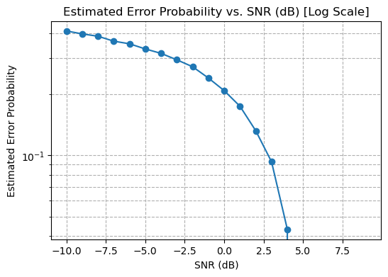
    plot_error_probability_vs_snr_log()
