MAP and ML Receivers, Decision Regions, and Error Probability#
Maximum a Posteriori Probability (MAP) Receivers#
The goal of an optimal receiver is to decide which message \( m \) was transmitted based on the observation of the received vector \(\vec{r}\). One common approach is to maximize the a posteriori probability, leading to the Maximum a Posteriori Probability (MAP) receiver, which we mentioned earlier, i.e.:
Bayes’ Rule#
Using Bayes’ Rule, the a posteriori probability of message \( m \) given the observation \(\vec{r}\) is
where:
\(P_m = \Pr(m)\) is the prior probability that the \(m\)-th message is transmitted,
\(p(\vec{r}|\vec{s}_m)\) is the likelihood function (i.e., the conditional probability density of observing \(\vec{r}\) given that the signal vector \(\vec{s}_m\) was sent), and
\(p(\vec{r})\) is the marginal probability density of the received vector \(\vec{r}\).
MAP Decision Rule#
The MAP decision rule selects the message that maximizes the posterior probability:
Substituting the expression from Bayes’ Rule, we have
Because the denominator \( p(\vec{r}) \) is independent of \( m \) (it is simply a normalizing constant ensuring that the probabilities sum to one), it does not affect the maximization. Thus, the decision rule can be simplified to
This formulation is particularly convenient because both the prior probabilities \( P_m \) and the likelihood \( p(\vec{r}|\vec{s}_m) \) are usually known or can be computed from the system model. In practice, the receiver computes the product \( P_m\, p(\vec{r}|\vec{s}_m) \) for each message \( m \) and selects the message corresponding to the largest value.
Maximum-Likelihood (ML) Receivers#
When designing a receiver, our objective is to decide which message \( m \) was transmitted based on the observed vector \(\vec{r}\). In general, the optimal decision rule according to the Maximum a Posteriori (MAP) criterion is given by \( \hat{m} = \underset{1 \leq m \leq M}{\arg\max}\, P_m \, p(\vec{r}|\vec{s}_m) \)
Equiprobable Messages#
In many practical systems, it is often assumed that the messages are equiprobable. This means that
Maximum-Likelihood (ML) Decision Rule#
When this assumption holds, the prior probability \( P_m \) becomes a constant across all messages. Since a constant factor does not affect the argmax operation, the MAP decision rule simplifies to
The term \( p(\vec{r}|\vec{s}_m) \) is known as the likelihood of message \( m \). Consequently, the decision rule that selects the message \( m \) with the highest likelihood is called the Maximum-Likelihood (ML) receiver.
Note that this rule is optimal (i.e., it minimizes the probability of error) only when all messages are equiprobable.
Decision Regions#
Output Space#
The output space \(\mathbb{R}^N\) represents the collection of all possible \(N\)-dimensional received signal vectors \(\vec{r}\).
Under an AWGN channel, where the noise is modeled as a continuous Gaussian random vector with infinite support, the output space \(\mathbb{R}^N\) is accordingly infinite. This means that there are infinitely many possible received vectors because the noise can take on any value in \(\mathbb{R}^N\).
In practice, even though the output space is infinite, detection algorithms work by partitioning this infinite space into decision regions (which are subsets of \(\mathbb{R}^N\)) to decide which of the \(M\) possible transmitted messages (or signal vectors) is most likely to have produced the observed \(\vec{r}\).
Decision Regions#
The receiver must decide which message was transmitted based on the observed received vector \(\vec{r}\) using a certain detector, e.g., a MAP (Maximum a Posteriori) or ML (Maximum Likelihood) detector.
The receiver partitions the output space, \(\mathbb{R}^N\), into \(M\) distinct regions. These regions are denoted as \(D_1, D_2, \ldots, D_M\).
Definition:
Let \( g: \mathbb{R}^N \to \{1, 2, \ldots, M\} \) be a decision function that maps each received \(N\)-dimensional vector \(\vec{r}\) to a message index. Then, the decision region for message \(m\), denoted by \( D_m \), is defined as
Each decision region \(D_m\) is the set of all possible outputs (or received vectors) that the detector maps to the message \(m\). In other words, \(D_m\) contains every \(\vec{r}\) for which the detector “believes” message \(m\) was transmitted.
Decision Mapping:
The basic idea is that if the received vector \(\vec{r}\) falls into a particular region \(D_m\), then the detector decides in favor of message \(m\); that is, the decision function \(g(\vec{r})\) yields\[ \hat{m} = g(\vec{r}) = m \quad \text{if } \vec{r} \in D_m \]
Example: Optimal Decision Regions for a MAP Detector#
For a MAP receiver, the decision region corresponding to message \(m\) is defined as
This expression means that if the received vector \(\vec{r}\) is such that the a posteriori probability \(\Pr[m|\vec{r}]\) is higher than the a posteriori probability for any other message \(m'\), then \(\vec{r}\) is assigned to \(D_m\), and the detector declares that message \(m\) was sent.
Ambiguities
It is possible that for some received vector \(\vec{r}\), two or more messages might achieve the same maximum a posteriori probability. In such cases, the detector can arbitrarily assign \(\vec{r}\) to one of the corresponding decision regions.
Discussion: Dependence of Infinite Output Space on Finite Set of Transmitted Signals#
Although the output space \(\mathbb{R}^N\) is infinite—since the additive noise (such as AWGN) can take any value and thus produces infinitely many possible received vectors—the received signals are statistically centered around the \(M\) finite signals used in the constellation at the transmitter. This finite set of transmitted signals fundamentally determines the structure of the received signals.
Infinite Output Space \(\mathbb{R}^N\):
The channel output is modeled as \(
\vec{r} = \vec{s}_m + \vec{n}\),
where \(\vec{s}_m\) is one of the \(M\) transmitted signal vectors and \(\vec{n}\) is a noise vector that can take any value in \(\mathbb{R}^N\) (because, for instance, Gaussian noise has infinite support). Thus, even though \(\vec{s}_m\) comes from a finite set, \(\vec{r}\) can be any vector in \(\mathbb{R}^N\).
Dependence on the Finite Set of Transmitted Signals:
The statistical distribution of \(\vec{r}\) is centered around the transmitted signal \(\vec{s}_m\). In other words, for a given transmitted signal, the likelihood function \(p(\vec{r}|\vec{s}_m)\) is maximized near \(\vec{s}_m\) and decays as \(\vec{r}\) moves away. This means that the bulk of the probability mass for \(\vec{r}\) when \(\vec{s}_m\) is transmitted is concentrated in a region surrounding \(\vec{s}_m\).
Determining Decision Regions:
Given the finite set of signals and the known noise statistics, we can define decision regions \(D_m\) in \(\mathbb{R}^N\). Each decision region \(D_m\) is the set of all received vectors that are “closer” (in a probabilistic sense) to the signal \(\vec{s}_m\) than to any other signal.
Discussion: Making Decision on New Received Signal#
The output space \(\mathbb{R}^N\) exists as the set of all possible received vectors, and the decision regions \(D_m\) are a predetermined partition of this space, designed according to the detection rule. When a new received signal arrives, it is simply mapped to one of these regions to make a decision.
Output Space \(\mathbb{R}^N\):
This is a mathematical model of all possible \(N\)-dimensional received signal vectors. It exists as a theoretical space that encompasses every possible outcome that the channel (e.g., an AWGN channel) might produce.
Decision Regions \(D_m\):
These regions are defined as a partition of the output space \(\mathbb{R}^N\) based on the detection rule (such as the MAP or ML rule). The decision regions are designed a priori—that is, before or independently of any particular received signal—based on the known or assumed statistical properties of the channel and the signal set. For example, in a MAP detector, each region \(D_m\) is defined as
The probabilities \(\Pr(m|\vec{r})\) and \(\Pr(m'|\vec{r})\) are computed using the statistical models of the channel and the prior information about the messages. Once these posterior probabilities are derived theoretically (typically via Bayes’ rule), the decision regions \(D_m\) can be determined. These regions are established based on the theoretical analysis of the channel’s statistics and are then used in the detection process for any new received signal.
Design and Usage
Design Time:
The decision regions are derived from the detection rule and are set up as part of the receiver design. They exist as fixed subsets of \(\mathbb{R}^N\).Run Time (New Observations):
When a new received signal \(\vec{r}\) comes in, the receiver doesn’t “redefine” the decision regions. Instead, it simply checks which region \(D_m\) the new \(\vec{r}\) falls into. The decision \( \hat{m} \) is then made accordingly.
Error Probability (Symbol Error Probability)#
When a message is transmitted over a channel, an error occurs if the received vector \(\vec{r}\) does not fall within the decision region corresponding to the transmitted message. Assume the transmitter sends the \(m\)th message, whose corresponding signal vector is \(\vec{s}_m\). The decision region for message \(m\) is denoted by \(D_m\). If \(\vec{r} \notin D_m\), then an error is declared.
Conditional Error Probability#
Define the conditional error probability \(P_{e|m}\) as the probability of making an error given that message \(m\) (or signal \(\vec{s}_m\)) is transmitted:
Since the decision regions \(\{D_m\}\) form a partition of the output space \(\mathbb{R}^N\), the complement of \(D_m\), denoted \(D_m^c\), is the union of the decision regions corresponding to all other messages. Thus, we can write:
where \(p(\vec{r}|\vec{s}_m)\) is the likelihood of receiving \(\vec{r}\) given that \(\vec{s}_m\) was transmitted.
Overall Error Probability#
Let \(P_m = \Pr(m)\) denote the prior probability that message \(m\) is transmitted. The overall symbol error probability \(P_e\) is the weighted sum of the conditional error probabilities over all messages:
Substituting the expression for \(P_{e|m}\), we obtain:
Proof#
The overall symbol error probability \( P_e \) is computed using the Total Probability Theorem.
Total Probability Theorem#
The Total Probability Theorem states that if \(\{A_m\}\) is a partition of the sample space, then for any event \(B\),
In the context of symbol error probability, the events \(A_m\) correspond to the different messages being transmitted, and the event \(B\) is the occurrence of an error (i.e., the receiver making an incorrect decision). Specifically:
\(A_m\): The event that message \( m \) is transmitted, which occurs with probability \( P_m = \Pr(m) \).
\(B\): The event that an error occurs, i.e., the received vector \(\vec{r}\) does not fall in the correct decision region \(D_m\).
Applying the Total Probability Theorem#
Using the Total Probability Theorem, the overall symbol error probability \( P_e \) is computed by summing the conditional error probabilities over all possible messages, weighted by the probability of each message being transmitted:
This completes the proof.
\(\blacksquare\)
Symbol Error Probability and Bit Error Probability#
Symbol Error Probability (\(P_e\)):
\(P_e\) is defined as the probability that a transmitted symbol (or message) is detected incorrectly at the receiver.
Bit Error Probability (\(P_b\)):
\(P_b\) is the probability that an individual bit is received in error.
Since each symbol typically represents a group of bits, a symbol error may result in one or more bit errors.
Challenges in Determining \(P_b\)#
Calculating \(P_b\) directly can be challenging because:
Mapping Dependency:
The bit error probability depends on the specific mapping between bits and signal points (or symbols), e.g., Gray coding.Constellation Symmetry:
In symmetric constellations, the structure of the constellation can simplify the calculation of \(P_b\). However, for arbitrary mappings or nonuniform constellations, the relationship may be more complex.
Bounds on \(P_b\)#
Consider a modulation scheme where each symbol represents \(k\) bits, so that the number of symbols is \(M = 2^k\). When a symbol error occurs, at least one bit error must occur. In the worst-case scenario, a symbol error might result in all \(k\) bits being in error. Therefore, the following bounds hold:
or, equivalently, since \(k = \log_2 M\):
Lower Bound (\(P_e/\log_2 M\)):
This bound corresponds to an ideal situation where, on average, a symbol error results in only one bit error. In many systems that use Gray coding, most symbol errors indeed lead to only a single bit error, making this bound a reasonable approximation for \(P_b\).Upper Bound (\(P_e\)):
This bound represents the worst-case scenario where every symbol error results in all \(k\) bits being erroneous.
This set of inequalities provides useful bounds on \(P_b\) when \(P_e\) is known, and vice versa. The exact relationship between \(P_e\) and \(P_b\) depends on the modulation format and the bit-to-symbol mapping, e.g., the channel coding schemes.
Example: Two Equiprobable Signals in Exponential Noise#
Consider two equiprobable message signals:
The channel adds independent noise components \(n_1\) and \(n_2\) to the transmitted signal. Each noise component has an exponential probability density function (PDF):
Since the noise components are independent, the joint PDF of the noise vector \(\vec{n} = (n_1, n_2)\) is
Maximum-Likelihood (ML) Detection#
Because the messages are equiprobable, the Maximum a Posteriori (MAP) detector reduces to the Maximum-Likelihood (ML) detector. The ML rule chooses the message \(m\) that maximizes the likelihood \(p(\vec{r}|\vec{s}_m)\). The decision region for message \(m\) is defined as
Since the received vector \(\vec{r}\) is given by
we can write
Determining the Decision Regions#
For \(\vec{s}_1 = (0,0)\):
The likelihood function is\[ p(\vec{r}|\vec{s}_1) = p(n_1 = r_1,\, n_2 = r_2) = e^{-r_1-r_2} \]provided \(r_1 \geq 0\) and \(r_2 \geq 0\).
For \(\vec{s}_2 = (1,1)\):
The likelihood is\[ p(\vec{r}|\vec{s}_2) = p(n_1 = r_1-1,\, n_2 = r_2-1) \]This is nonzero only if \(r_1-1 \ge 0\) and \(r_2-1 \ge 0\); that is, when \(r_1 \geq 1\) and \(r_2 \geq 1\). In this case,
\[ p(\vec{r}|\vec{s}_2) = e^{-(r_1-1)-(r_2-1)} = e^{-r_1-r_2+2} \]Comparison of Likelihoods:
If either \(r_1 < 1\) or \(r_2 < 1\):
For such \(\vec{r}\), note that at least one of \(r_1-1\) or \(r_2-1\) is negative, which makes \(p(\vec{r}|\vec{s}_2) = 0\) (because the noise PDF is zero for negative arguments). However, \(p(\vec{r}|\vec{s}_1)\) is positive (since \(r_1, r_2 \ge 0\)). Therefore, when either coordinate is less than 1, we have\[ p(\vec{r}|\vec{s}_1) > p(\vec{r}|\vec{s}_2) \]and the ML detector will decide in favor of message 1. Thus,
\[ D_1 \supset \{ \vec{r} \in \mathbb{R}^2 : r_1 \ge 0,\; r_2 \ge 0,\; \text{and either } r_1 < 1 \text{ or } r_2 < 1 \} \]If \(r_1 \geq 1\) and \(r_2 \geq 1\):
Both likelihoods are positive. In this region,\[ p(\vec{r}|\vec{s}_1) = e^{-r_1-r_2} \quad \text{and} \quad p(\vec{r}|\vec{s}_2) = e^{-r_1-r_2+2} \]Since \(e^{-r_1-r_2+2} = e^2 \, e^{-r_1-r_2}\) and \(e^2 > 1\), it follows that
\[ p(\vec{r}|\vec{s}_2) > p(\vec{r}|\vec{s}_1) \]Hence, for \(\vec{r}\) satisfying \(r_1 \geq 1\) and \(r_2 \geq 1\), the ML detector selects message 2. Thus,
\[ D_2 = \{ \vec{r} \in \mathbb{R}^2 : r_1 \geq 1,\; r_2 \geq 1 \} \]
Thus, we have the decision regions are:
Error Probability Calculation#
Since the messages are equiprobable, the probability of error is determined by the event that an error occurs when message 1 is transmitted (because an error only occurs when \(\vec{s}_1\) is sent and the received vector falls in \(D_2\)). That is,
When \(\vec{s}_1 = (0,0)\) is transmitted, the received vector is
with \(n_1\) and \(n_2\) being independent and exponentially distributed. The event \(\vec{r} \in D_2\) corresponds to
For an exponential random variable with PDF \(e^{-n}\) for \(n \geq 0\), the probability that \(n \geq 1\) is
Because \(n_1\) and \(n_2\) are independent,
Thus, the error probability is
\(\square\)
Simulation#
import numpy as np
import matplotlib.pyplot as plt
from matplotlib.patches import Rectangle
from matplotlib.lines import Line2D

# Parameters for Monte-Carlo Simulation
num_trials = 100000  # Number of trials
s1 = np.array([0, 0])
s2 = np.array([1, 1])
theoretical_pe = 0.5 * np.exp(-2)  # Theoretical P_e = 1/2 * e^(-2)

# Monte-Carlo Simulation
np.random.seed(42)  # For reproducibility
transmitted = np.random.choice([0, 1], size=num_trials, p=[0.5, 0.5])  # 0 for s1, 1 for s2
errors = 0
r_points_s1 = []  # Store received points for plotting (s1 transmitted)
r_points_s2 = []  # Store received points for plotting (s2 transmitted)

for i in range(num_trials):
    noise = np.random.exponential(scale=1, size=2)  # [n1, n2]
    if transmitted[i] == 0:
        s = s1
        r_points_s1.append(s + noise)
    else:
        s = s2
        r_points_s2.append(s + noise)
    r = s + noise
    decided = 0 if (r[0] < 1 or r[1] < 1) else 1  # ML Decision Rule
    if decided != transmitted[i]:
        errors += 1

simulated_pe = errors / num_trials
print(f"Theoretical P_e: {theoretical_pe:.5f}")
print(f"Simulated P_e: {simulated_pe:.5f}")
print(f"Absolute difference: {abs(theoretical_pe - simulated_pe):.5f}")
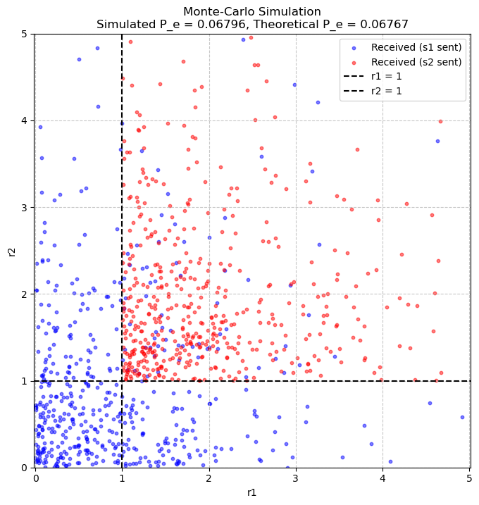
Theoretical P_e: 0.06767
Simulated P_e: 0.06796
Absolute difference: 0.00029
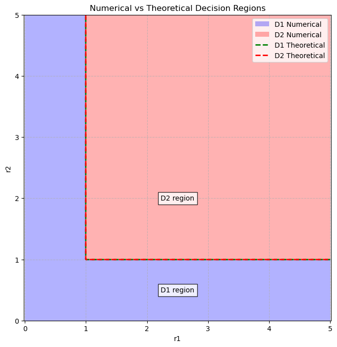
# Separate Decision Regions Plot
def noise_pdf(n):
    return np.where(n >= 0, np.exp(-n), 0)

# Create grid for decision regions
r1_values = np.linspace(0, 5, 500)  # Match Monte-Carlo plot range
r2_values = np.linspace(0, 5, 500)
R1, R2 = np.meshgrid(r1_values, r2_values)

# Numerical decision regions
p_r_given_s1 = noise_pdf(R1) * noise_pdf(R2)
p_r_given_s2 = noise_pdf(R1 - 1) * noise_pdf(R2 - 1)
D1_numerical = p_r_given_s1 > p_r_given_s2
D2_numerical = (R1 >= 1) & (R2 >= 1)

# Theoretical decision regions
D1_theoretical = np.logical_or(R1 < 1, R2 < 1) & (R1 >= 0) & (R2 >= 0)
D2_theoretical = (R1 >= 1) & (R2 >= 1)

# Plot decision regions
plt.figure(figsize=(8, 8))
plt.contourf(R1, R2, D1_numerical, levels=[0.5, 1], colors='blue', alpha=0.3)
plt.contourf(R1, R2, D2_numerical, levels=[0.5, 1], colors='red', alpha=0.3)
plt.contour(R1, R2, D1_theoretical, levels=[0.5], colors='green', linestyles='--', linewidths=2)
plt.contour(R1, R2, D2_theoretical, levels=[0.5], colors='red', linestyles='--', linewidths=2)

# Customize plot
plt.xlabel('r1')
plt.ylabel('r2')
plt.title('Numerical vs Theoretical Decision Regions')
plt.axis('equal')
plt.xlim(0, 5)
plt.ylim(0, 5)
plt.grid(True, linestyle='--', alpha=0.7)

# Add annotations
mid_value = np.mean([r1_values.min(), r1_values.max()])
plt.text(mid_value, 0.5, 'D1 region', ha='center', va='center',
         bbox=dict(facecolor='white', alpha=0.8))
plt.text(mid_value, 2, 'D2 region', ha='center', va='center',
         bbox=dict(facecolor='white', alpha=0.8))

# Legend proxies
proxies = [
    Rectangle((0, 0), 1, 1, facecolor='blue', alpha=0.3),
    Rectangle((0, 0), 1, 1, facecolor='red', alpha=0.3),
    Line2D([0], [0], color='green', linestyle='--', linewidth=2),
    Line2D([0], [0], color='red', linestyle='--', linewidth=2)
]
plt.legend(proxies, ['D1 Numerical', 'D2 Numerical', 'D1 Theoretical', 'D2 Theoretical'], loc='upper right')

plt.show()
# Monte-Carlo Plot
subset_size = 500
r1_s1 = [p[0] for p in r_points_s1[:subset_size]]
r2_s1 = [p[1] for p in r_points_s1[:subset_size]]
r1_s2 = [p[0] for p in r_points_s2[:subset_size]]
r2_s2 = [p[1] for p in r_points_s2[:subset_size]]

plt.figure(figsize=(8, 8))
plt.scatter(r1_s1, r2_s1, color='blue', alpha=0.5, label='Received (s1 sent)', s=10)
plt.scatter(r1_s2, r2_s2, color='red', alpha=0.5, label='Received (s2 sent)', s=10)
plt.axvline(x=1, color='black', linestyle='--', label='r1 = 1')
plt.axhline(y=1, color='black', linestyle='--', label='r2 = 1')
plt.xlabel('r1')
plt.ylabel('r2')
plt.title(f'Monte-Carlo Simulation\nSimulated P_e = {simulated_pe:.5f}, Theoretical P_e = {theoretical_pe:.5f}')
plt.axis('equal')
plt.legend()
plt.grid(True, linestyle='--', alpha=0.7)
plt.xlim(0, 5)
plt.ylim(0, 5)
plt.show()