Signal Space

Signal Space Concepts

Inner Product of Complex Signals

The inner product of two complex-valued signals, \( x_1(t) \) and \( x_2(t) \), is defined as:

\[ \langle x_1(t), x_2(t) \rangle = \int_{-\infty}^{\infty} x_1(t) x_2^*(t) \, dt \]

Here, \( x_2^*(t) \) denotes the complex conjugate of \( x_2(t) \).

Orthogonal Signals

Two signals are considered orthogonal if their inner product is zero:

\[ \langle x_1(t), x_2(t) \rangle = 0 \]

Orthonormal Signals

A set of \( m \) signals is orthonormal if:

1. The signals are mutually orthogonal.

2. Each signal has a norm of 1 (unit length).

Norm and Signal Energy

The norm of a signal \( x(t) \) is defined as:

\[ \|x(t)\| = \sqrt{\int_{-\infty}^{\infty} |x(t)|^2 \, dt} = \sqrt{\mathcal{E}_x} \]

Here, \( \mathcal{E}_x \) represents the total energy of the signal \( x(t) \).

Linearly Independent Signals

A set of \( m \) signals is considered linearly independent if no signal in the set can be expressed as a linear combination of the other signals.

Python Example: Orthonormal Signals

import numpy as np
import matplotlib.pyplot as plt

# Define the simulation parameters
Fs = 1000  # Sampling frequency in Hz
T = 1      # Duration of the signal in seconds
t = np.arange(0, T, 1/Fs)  # Time vector for one second worth of samples

# Define two signals
f = 5  # Common frequency
x1 = np.sin(2 * np.pi * f * t)  # First signal: sine wave
x2 = np.cos(2 * np.pi * f * t)  # Second signal: cosine wave (orthogonal to sine)

# Compute the norms (energy) of the signals
norm_x1 = np.sqrt(np.trapz(x1**2, t))
norm_x2 = np.sqrt(np.trapz(x2**2, t))

# Normalize the signals
x1_normalized = x1 / norm_x1
x2_normalized = x2 / norm_x2

# Compute the inner product of normalized signals
inner_product = np.trapz(x1_normalized * x2_normalized, t)

# Plot the signals
plt.figure(figsize=(12, 6))

# Plot x1(t)
plt.subplot(2, 1, 1)
plt.plot(t, x1_normalized, linewidth=2, label=f'Normalized x1(t) = sin(2π{f}t)')
plt.title('Normalized Signal x1(t)')
plt.xlabel('Time (s)')
plt.ylabel('Amplitude')
plt.grid(True)
plt.legend()

# Plot x2(t)
plt.subplot(2, 1, 2)
plt.plot(t, x2_normalized, linewidth=2, label=f'Normalized x2(t) = cos(2π{f}t)')
plt.title('Normalized Signal x2(t)')
plt.xlabel('Time (s)')
plt.ylabel('Amplitude')
plt.grid(True)
plt.legend()

# Show the plots
plt.tight_layout()
plt.show()

# Output the results
print(f"The norm of normalized x1(t) is: {np.sqrt(np.trapz(x1_normalized**2, t)):.6f}")
print(f"The norm of normalized x2(t) is: {np.sqrt(np.trapz(x2_normalized**2, t)):.6f}")
print(f"The inner product of the normalized signals is: {inner_product:.6f}")

# Check orthonormality
tolerance = 1e-3  # Tolerance for numerical precision
is_x1_normalized = abs(np.sqrt(np.trapz(x1_normalized**2, t)) - 1) < tolerance
is_x2_normalized = abs(np.sqrt(np.trapz(x2_normalized**2, t)) - 1) < tolerance
is_orthogonal = abs(inner_product) < tolerance

if is_x1_normalized and is_x2_normalized and is_orthogonal:
    print("The signals are orthonormal.")
else:
    print("The signals are not orthonormal.")

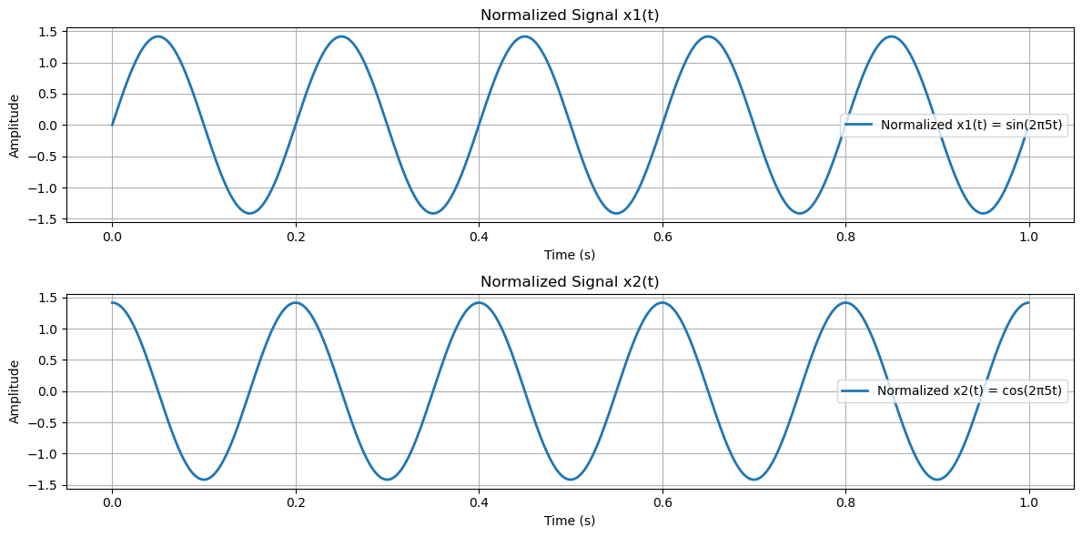
The norm of normalized x1(t) is: 1.000000
The norm of normalized x2(t) is: 1.000000
The inner product of the normalized signals is: 0.000031
The signals are orthonormal.

Some Important Inequalities

Triangle Inequality

For two signals \( x_1(t) \) and \( x_2(t) \), the triangle inequality states:

\[ \|x_1(t) + x_2(t)\| \leq \|x_1(t)\| + \|x_2(t)\| \]

This inequality highlights that the norm of the sum of two signals is never greater than the sum of their individual norms.

Cauchy–Schwarz Inequality

The Cauchy–Schwarz inequality is a fundamental result that applies to the inner product of two signals \( x_1(t) \) and \( x_2(t) \):

\[ |\langle x_1(t), x_2(t) \rangle| \leq \|x_1(t)\| \cdot \|x_2(t)\| = \sqrt{\mathcal{E}_{x_1} \mathcal{E}_{x_2}} \]

Equivalently, in integral form:

\[ \left| \int_{-\infty}^{\infty} x_1(t) x_2^*(t) \, dt \right| \leq \sqrt{\int_{-\infty}^{\infty} |x_1(t)|^2 \, dt} \cdot \sqrt{\int_{-\infty}^{\infty} |x_2(t)|^2 \, dt} \]

Equality holds in the Cauchy–Schwarz inequality if and only if \( x_2(t) = a x_1(t) \), where \( a \) is any complex scalar.

Orthogonal Expansions of Signals

Vector Representation of Signals

We can represent signal waveforms as vectors, demonstrating the equivalence between a signal waveform and its vector representation.

Let \( s(t) \) be a deterministic signal with finite energy:

\[ \mathcal{E}_s = \int_{-\infty}^{\infty} |s(t)|^2 dt \]

Suppose there exists a set of orthonormal functions \( \{\phi_n(t)\}, n = 1, 2, ..., K \), such that:

\[\begin{split} \langle \phi_n(t), \phi_m(t) \rangle = \int_{-\infty}^{\infty} \phi_n(t) \phi_m^*(t) dt = \begin{cases} 1 & \text{if } n = m \\ 0 & \text{if } n \neq m \end{cases} \end{split}\]

Approximation of Signals

The signal \( s(t) \) can be approximated as a weighted linear combination of these orthonormal functions:

\[ \hat{s}(t) = \sum_{k=1}^{K} s_k \phi_k(t) \]

Here, \( \{s_k\} \) are the coefficients representing the projection of \( s(t) \) onto the functions \( \{\phi_k(t)\} \).

The approximation error is given by:

\[ e(t) = s(t) - \hat{s}(t) \]

Minimizing the Approximation Error

The energy of the approximation error is:

\[ \mathcal{E}_e = \int_{-\infty}^{\infty} |s(t) - \hat{s}(t)|^2 dt = \int_{-\infty}^{\infty} \left| s(t) - \sum_{k=1}^{K} s_k \phi_k(t) \right|^2 dt \]

To minimize \( \mathcal{E}_e \), the coefficients \( \{s_k\} \) are chosen such that \( \hat{s}(t) \) is the projection of \( s(t) \) onto the \( K \)-dimensional signal space spanned by \( \{\phi_k(t)\} \). In this case:

\[ \langle e(t), \hat{s}(t) \rangle = 0 \]

The minimum mean-square approximation error is:

\[ \mathcal{E}_{\text{min}} = \mathcal{E}_s - \sum_{k=1}^{K} |s_k|^2 \]

This value is always nonnegative by definition.

Perfect Representation of Signals

When the minimum mean-square error is zero (\( \mathcal{E}_{\text{min}} = 0 \)), we have:

\[ \mathcal{E}_s = \sum_{k=1}^{K} |s_k|^2 = \int_{-\infty}^{\infty} |s(t)|^2 dt \]

Under this condition, \( s(t) \) can be expressed as:

\[ s(t) = \sum_{k=1}^{K} s_k \phi_k(t) \]

This equality implies that \( s(t) \) is exactly represented by the series expansion, with no approximation error.

Complete Set of Orthonormal Functions

Definition
A set of orthonormal functions \( \{\phi_n(t)\} \) is said to be complete if every finite-energy signal \( s(t) \) can be represented as:

\[ s(t) = \sum_{k=1}^{K} s_k \phi_k(t) \]

with \( \mathcal{E}_{\text{min}} = 0 \).

Example: Trigonometric Fourier Series

A Fourier series is a mathematical representation of a signal as a sum of sine and cosine functions. The idea is to decompose a signal \( s(t) \), defined over a finite interval \( [0, T] \), into its frequency components.

Signal Decomposition

The signal \( s(t) \) can be expressed as:

\[ s(t) = \sum_{k=0}^{\infty} \left( a_k \cos \frac{2\pi kt}{T} + b_k \sin \frac{2\pi kt}{T} \right) \]

where:

• \( \cos \frac{2\pi kt}{T} \) and \( \sin \frac{2\pi kt}{T} \) are the basis functions representing periodic oscillations.

• \( a_k \) and \( b_k \) are the Fourier coefficients that determine the contribution of each cosine and sine term.

Fourier Coefficients

The Fourier coefficients \( a_k \) and \( b_k \) are derived to minimize the mean-square error, ensuring that the series closely approximates the original signal. They are calculated using:

• Constant term (DC component):

  \[ a_0 = \frac{1}{T} \int_{0}^{T} s(t) \, dt \]

  This represents the average (mean) value of the signal over \( [0, T] \).

• Cosine coefficients:

  \[ a_k = \frac{2}{T} \int_{0}^{T} s(t) \cos \frac{2\pi kt}{T} \, dt \quad \text{for } k = 1, 2, 3, \ldots \]

  These coefficients capture the contribution of cosine terms at different frequencies \( k/T \).

• Sine coefficients:

  \[ b_k = \frac{2}{T} \int_{0}^{T} s(t) \sin \frac{2\pi kt}{T} \, dt \quad \text{for } k = 1, 2, 3, \ldots \]

  These coefficients capture the contribution of sine terms at different frequencies \( k/T \).

Physical Interpretation

• The trigonometric Fourier series reveals the frequency components (harmonics) of the signal.

• \( a_0 \): Represents the average value of the signal.

• \( a_k \): Amplitudes of the cosine components at different frequencies.

• \( b_k \): Amplitudes of the sine components at different frequencies.

By combining these coefficients, we can reconstruct the original signal or analyze its frequency content.

Complete Basis Set
The functions:

\[ \left\{ \frac{1}{\sqrt{T}}, \sqrt{\frac{2}{T}} \cos \frac{2\pi kt}{T}, \sqrt{\frac{2}{T}} \sin \frac{2\pi kt}{T} \right\} \]

form a complete orthonormal set over the interval \( [0, T] \), which means:

1. Any periodic signal (with the required properties) can be represented as a linear combination of these functions.

2. The approximation error vanishes as more terms are included, achieving zero mean-square error in the limit.

Python Simulation

import numpy as np
import matplotlib.pyplot as plt

# Parameters
T = 1.0               # Duration (seconds)
fs = 1000             # Sampling rate (samples per second)
K = 100                # Number of harmonics
samples = int(fs * T) # Total number of samples
t = np.linspace(0, T, samples, endpoint=False) # Time vector

# Generate a square wave signal
square_wave = np.sign(np.sin(2 * np.pi * t / T))

# Compute Fourier coefficients
a0 = np.mean(square_wave)  # DC component
ak = []
bk = []

for k in range(1, K + 1):
    ak.append((2 / T) * np.sum(square_wave * np.cos(2 * np.pi * k * t / T)) / fs)
    bk.append((2 / T) * np.sum(square_wave * np.sin(2 * np.pi * k * t / T)) / fs)

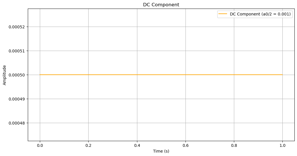
The Fourier series components

DC Component: The constant offset (\( a_0/2 \)) is displayed in the first subplot.

# DC Component

plt.figure(figsize=(12, 6))
plt.plot(t, np.full_like(t, a0 / 2), label=f"DC Component (a0/2 = {a0/2:.3f})", color='orange')
plt.xlabel("Time (s)")
plt.ylabel("Amplitude")
plt.title("DC Component")
plt.legend()
plt.grid()

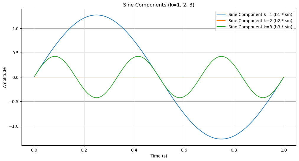
Sine Components: The sine terms (\( b_k \sin(2\pi kt / T) \)) for \( k = 1, 2, 3 \)

Note that, for \( b_k \):

\[ b_k = \frac{2}{T} \int_0^T s(t) \sin\left(\frac{2\pi k t}{T}\right) \, dt \]

For \( k = 2 \) (or any even \( k \)), the square wave alternates in such a way that the positive and negative parts of the sine wave cancel each other out perfectly, resulting in:

\[ b_2 = 0 \]

Generalized Consequence

• \( b_k \) is zero for all even \( k \), so the sine components for even \( k \) do not contribute to the signal.

• The observed “line” is likely just the \( y = 0 \) line, which corresponds to the sine component’s absence for \( k = 2 \).

# Sine Components for K = 1, 2, 3
plt.figure(figsize=(12, 6))
for k in range(1, 4):
    sine_component = bk[k - 1] * np.sin(2 * np.pi * k * t / T)
    plt.plot(t, sine_component, label=f"Sine Component k={k} (b{k} * sin)")
plt.xlabel("Time (s)")
plt.ylabel("Amplitude")
plt.title("Sine Components (k=1, 2, 3)")
plt.legend()
plt.grid()

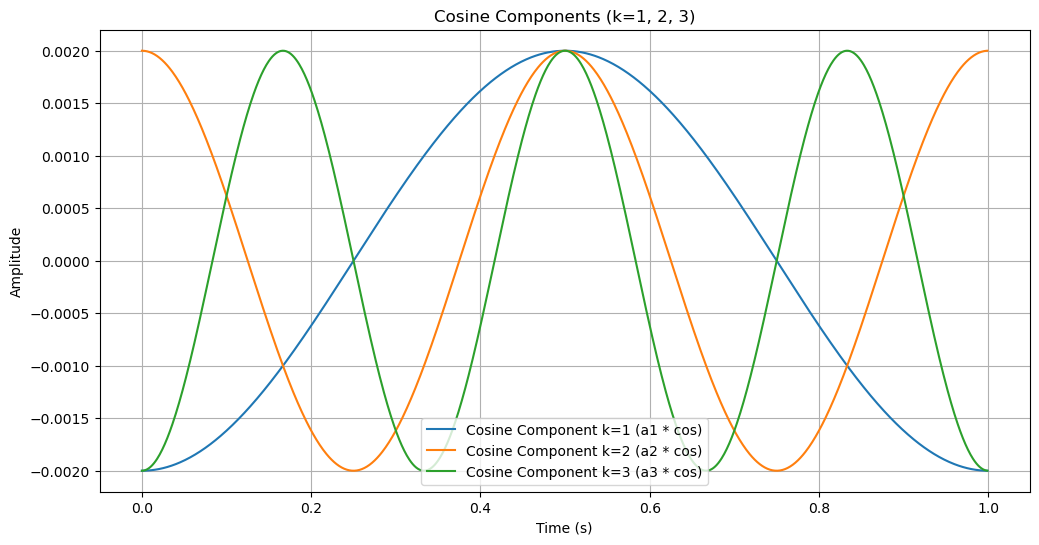
Cosine Components: The cosine terms (\( a_k \cos(2\pi kt / T) \)) for \( k = 1, 2, 3 \)

# Cosine Components for K = 1, 2, 3
plt.figure(figsize=(12, 6))
for k in range(1, 4):
    cosine_component = ak[k - 1] * np.cos(2 * np.pi * k * t / T)
    plt.plot(t, cosine_component, label=f"Cosine Component k={k} (a{k} * cos)")
plt.xlabel("Time (s)")
plt.ylabel("Amplitude")
plt.title("Cosine Components (k=1, 2, 3)")
plt.legend()
plt.grid()

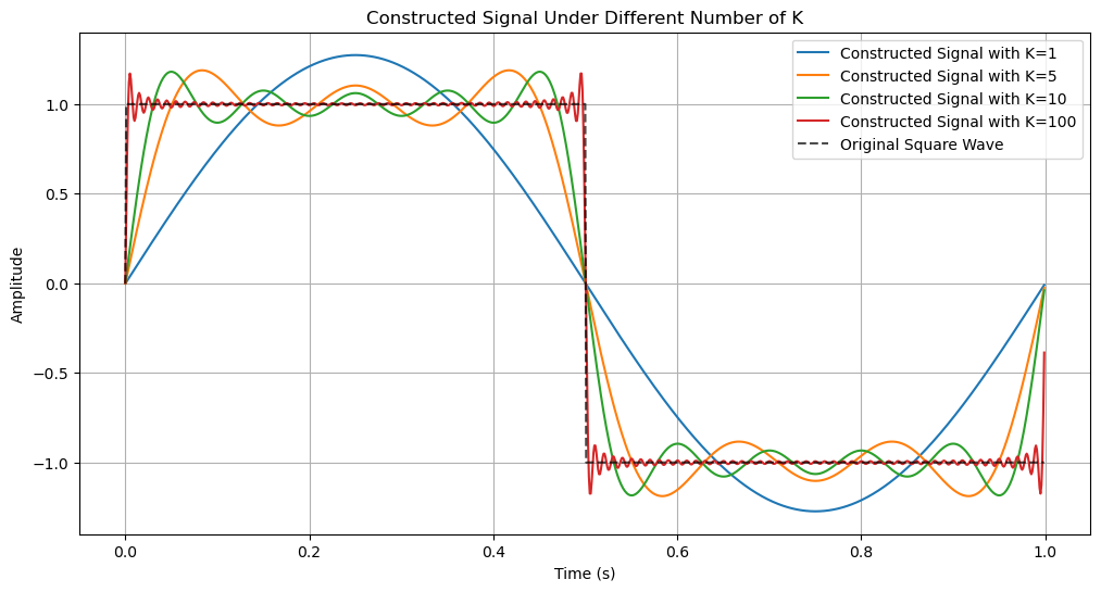
# Construct signal s(t) based on Fourier series
constructed_signals = []

for k_max in [1, 5, 10, K]:  # Different numbers of harmonics
    s_t = a0 / 2  # Initialize with DC component
    for k in range(1, k_max + 1):
        s_t += ak[k - 1] * np.cos(2 * np.pi * k * t / T) + bk[k - 1] * np.sin(2 * np.pi * k * t / T)
    constructed_signals.append((k_max, s_t))

# Plot constructed signal for different numbers of K
plt.figure(figsize=(12, 6))
for k_max, s_t in constructed_signals:
    plt.plot(t, s_t, label=f"Constructed Signal with K={k_max}")
plt.plot(t, square_wave, 'k--', label="Original Square Wave", alpha=0.7)
plt.xlabel("Time (s)")
plt.ylabel("Amplitude")
plt.title("Constructed Signal Under Different Number of K")
plt.legend()
plt.grid()
plt.show()

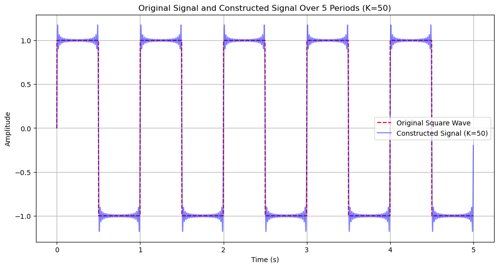
# Parameters for extended time range
periods = 5  # Number of periods to plot
t_extended = np.linspace(0, T * periods, samples * periods, endpoint=False)  # Extended time vector

# Generate the extended square wave signal
square_wave_extended = np.sign(np.sin(2 * np.pi * t_extended / T))

# Construct the signal with K = 100 harmonics
K_max = 50
a0_extended = np.mean(square_wave)  # DC component
s_t_extended = a0_extended / 2  # Start with the DC component
for k in range(1, K_max + 1):
    s_t_extended += (
        ak[k - 1] * np.cos(2 * np.pi * k * t_extended / T)
        + bk[k - 1] * np.sin(2 * np.pi * k * t_extended / T)
    )

# Plot the original signal and the constructed signal
plt.figure(figsize=(12, 6))
plt.plot(t_extended, square_wave_extended, label="Original Square Wave", linestyle="--", color="red")
plt.plot(t_extended, s_t_extended, label=f"Constructed Signal (K={K_max})", color="blue", alpha=0.5)
plt.xlabel("Time (s)")
plt.ylabel("Amplitude")
plt.title(f"Original Signal and Constructed Signal Over {periods} Periods (K={K_max})")
plt.legend()
plt.grid()
plt.show()