Efficient Receiver#
Sufficient Statistics#
In signal detection problems, the receiver observes a set of data or measurements that we can group into different components. Suppose that we label these components as \(\vec{r}_1\) and \(\vec{r}_2\), so that the overall received data can be written as \(\vec{r} = (\vec{r}_1, \vec{r}_2)\).
Markov Chain#
We consider a communication scenario in which a transmitter sends one of \(M\) possible signals, denoted by \(s_m\). Our goal at the receiver is to decide which \(s_m\) was sent based on the observed data \(\vec{r}\). One way to formalize the relationship between \(s_m\) and \((\vec{r}_1, \vec{r}_2)\) is through the assumption that
This factorization implies that \(s_m\), \(\vec{r}_1\), and \(\vec{r}_2\) form a Markov chain in the order \(s_m \to \vec{r}_1 \to \vec{r}_2\). Intuitively, once \(\vec{r}_1\) is known, the statistical relationship to \(\vec{r}_2\) no longer depends on the specific signal \(s_m\).
Detection and Decision Rule#
Let us denote the probability of sending signal \(s_m\) by \(P_m\). In a maximum a posteriori (MAP) detection framework, we seek to choose the signal \(\hat{m}\) that maximizes the posterior probability of \(s_m\) given the observation \(\vec{r}\). Equivalently, we often write a decision rule in terms of the joint probability:
By substituting \(\vec{r} = (\vec{r}_1, \vec{r}_2)\) and using our Markov chain assumption, this becomes:
Notice that \(p(\vec{r}_2 \mid \vec{r}_1)\) does not depend on which signal \(s_m\) was sent (once \(\vec{r}_1\) is given). It is thus a common factor for all \(m\) in the maximization and can be ignored in the decision rule. Therefore, the decision rule simplifies to:
This simplification reveals that only \(\vec{r}_1\) influences which \(s_m\) is selected. In other words, \(\vec{r}_2\) is irrelevant for the decision, given \(\vec{r}_1\).
Sufficient Statistics and Irrelevant Data#
When the factorization
holds, we say that \(\vec{r}_1\) is a sufficient statistic for detecting \(s_m\). A sufficient statistic is any function or part of the observed data from which we can make an optimal decision without losing any performance compared to using the full data set.
In this scenario, \(\vec{r}_2\) is called irrelevant data (or irrelevant information), because it does not affect the final decision about \(s_m\) once \(\vec{r}_1\) is known. Recognizing that \(\vec{r}_2\) is irrelevant means that we do not need to process or store it for detection purposes, thereby reducing receiver complexity and potentially saving computational and storage resources.
Importance in System Design#
In practice, identifying sufficient statistics enables a more efficient receiver design. If we know that part of the received data is irrelevant for detection, we can ignore or discard it early in the process—this often lowers the dimensionality of the problem and the cost of subsequent processing. Engineers and system designers leverage this concept to build simplified detectors that still maintain the same optimal performance as if they used all the data.
Sufficient Statistics in Example: Two Equiprobable Signals in Exponential Noise#
In this example, the receiver only observes the two-dimensional signal \(\vec{r} = (r_1, r_2)\). Here, we augment the observation so that the receiver also directly observes the noise component \(n_1\). Thus, the total observed data can be denoted by \(\vec{r} = (\vec{r}_1, \vec{r}_2)\), where
\(\vec{r}_1 = (r_1, n_1)\)
\(\vec{r}_2 = r_2.\)
Augmented Observation Changes Detection#
Recall that the transmitted messages are:
When message \(m\) is sent, the received signal is:
For \(m = 1\), \(s_{11} = 0\) and \(s_{12} = 0\).
For \(m = 2\), \(s_{21} = 1\) and \(s_{22} = 1\).
By observing both \(r_1\) and \(n_1\), the receiver effectively knows:
Since \(s_{11} = 0\) and \(s_{21} = 1\), knowledge of \(r_1 - n_1\) directly reveals which message was sent:
If \(r_1 - n_1 = 0\), then \(m = 1\).
If \(r_1 - n_1 = 1\), then \(m = 2\).
With this direct determination of \(m\), the value of \(r_2\) no longer matters for the detection decision. In other words, once \(\vec{r}_1 = (r_1, n_1)\) is known, the probability distribution of \(r_2\) does not affect the message decision. The set \(\vec{r}_1\) is therefore a sufficient statistic for deciding whether \(m = 1\) or \(m = 2\).
Irrelevant Data#
Because \(\vec{r}_1\) completely determines the transmitted message, \(\vec{r}_2 = r_2\) is irrelevant to the detection. Formally, this means
so once \(\vec{r}_1\) is known, further knowledge of \(s_m\) does not change the distribution of \(r_2\). As a result, including \(r_2\) in the detection rule cannot improve performance.
In this modified scenario, \(\vec{r}_1 = (r_1, n_1)\) is sufficient because it alone reveals which message was sent. Thus, \(\vec{r}_2 = r_2\) can be disregarded.
Decision Rule and Error Probability#
Since \(r_1 - n_1\) perfectly reveals which message was sent, the optimal decision rule becomes:
Under this scheme, there is no overlap between the outcomes corresponding to \(m=1\) and \(m=2\). Consequently, the error probability is zero.
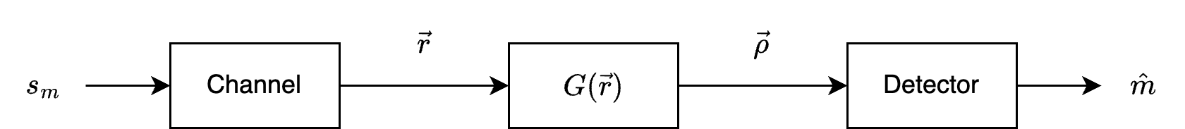
Preprocessing at the Receiver#
In many communication systems, the received signal vector \(\vec{r}\) may be subjected to transformations before being passed to the detector. This process is known as preprocessing, and it is often used to simplify or improve subsequent detection tasks. A key point is that if the preprocessing operation is invertible, it does not affect the ultimate performance of the optimal detector.
Invertible Transformation#
Suppose the receiver applies an invertible function (or transformation) \( G(\cdot) \) to the received vector \(\vec{r}\). The output of this transformation is:
Because \(G(\cdot)\) is invertible, we can recover \(\vec{r}\) exactly from \(\vec{\rho}\) by applying the inverse transformation \(G^{-1}(\cdot)\). Hence,
Therefore, once \(\vec{\rho}\) is available, \(\vec{r}\) is also effectively available (via \(G^{-1}\)). The detector can then use both \(\vec{r}\) and \(\vec{\rho}\) if needed.
Effect on the Detection Rule#
To see why preprocessing with an invertible transformation does not alter optimality, let us consider the standard form of the maximum a posteriori (MAP) or maximum-likelihood (ML) decision rule. When \(\vec{\rho}\) is supplied to the detector, the optimal decision is:
Using the fact that \(\vec{\rho} = G(\vec{r})\) depends solely on \(\vec{r}\) (and not directly on \(s_m\)), we factorize:
But since \(\vec{\rho}\) is uniquely determined by \(\vec{r}\), the conditional probability \(p(\vec{\rho} \mid \vec{r})\) does not depend on which signal \(s_m\) was sent. This term is effectively a constant with respect to \(m\). Therefore, maximizing over \(m\) is equivalent to:
Thus, whether the detector works with \(\vec{r}\) directly or first transforms \(\vec{r}\) to \(\vec{\rho} = G(\vec{r})\), the same detection rule applies, yielding the same decision. In other words, an invertible preprocessing does not degrade or change the optimal detection performance.
Example: Whitening Filter#
A common application of invertible preprocessing arises when the noise in the channel is colored, meaning its components are correlated or have frequency-dependent power. Suppose the received vector is
where \(\vec{n}\) is a nonwhite (colored) noise vector. If there exists an invertible operator (matrix) \(W\) that can “whiten” the noise, we define a new variable:
If \(\vec{v}\) is white noise (uncorrelated components with identical variance), then we can rewrite:
This transformed system looks like a channel with white noise, which is often simpler to analyze. Importantly, because \(W\) is an invertible linear transformation, no information is lost, and the optimal detection performance remains unchanged. In practice, applying \(W\) before detection is called whitening, and the matrix \(W\) is referred to as a whitening filter.