Multidimensional Signaling

Multidimensional signaling is a powerful technique used in digital communication systems to enhance the efficient transmission of information. By representing signals as vectors in higher-dimensional spaces, it becomes possible to pack more data into each transmission interval, improving bandwidth utilization and overall system performance.

Specifically, in digital communication, a signal is often represented as a vector whose components correspond to different dimensions. These dimensions can be defined in various domains, such as time and frequency. By increasing the number of dimensions, the signal can carry more information, which results in more efficient use of the communication channel.

Time Division

• Time Interval Subdivision: Consider a total time interval \( T_1 \) that is subdivided into \( N \) smaller subintervals, each of duration \( T = \frac{T_1}{N} \).

• Component Transmission: In each subinterval, one component of an \( N \)-dimensional signal vector is transmitted. A common modulation technique used in this context is binary Pulse Amplitude Modulation (PAM), which represents data as one of two amplitude levels.

By subdividing time in this manner, each segment carries a distinct component of the overall signal vector, effectively mapping the transmission into an \( N \)-dimensional space.

Quadrature Modulation Technique

• Even-Dimensional Signal Vectors: If \( N \) is even, the signal can be divided such that two components are transmitted simultaneously within each time slot.

• Quadrature Carriers: This simultaneous transmission is achieved by modulating two sinusoidal carriers that are 90 degrees out of phase with each other (often referred to as in-phase and quadrature-phase carriers). This method, known as Quadrature Amplitude Modulation (QAM), enables the communication system to send twice as many components in the same time slot compared to using a single carrier.

Frequency Division

• Frequency Band Division: A frequency band with total width \( N \Delta f \) can be divided into \( N \) discrete frequency slots, each of width \( \Delta f \).

• Frequency Domain Transmission: Each frequency slot is used to transmit one component of the \( N \)-dimensional signal vector by modulating the amplitude of a carrier at the designated frequency.

• No Cross-Talk: The proper spacing of \( \Delta f \) between frequency slots ensures that the carriers do not interfere with one another, eliminating cross-talk.

Hybrid Time and Frequency Utilization

• Quadrature Carriers in Frequency Slots: When quadrature carriers are employed in the frequency domain, an \( N \)-dimensional signal vector can be transmitted over \( \frac{N}{2} \) frequency slots. This technique effectively doubles the bandwidth utilization, as each slot carries two dimensions of the signal.

• Joint Time-Frequency Signaling: By combining time and frequency domain techniques, a higher-dimensional signal vector can be transmitted efficiently. This joint use allows for even more flexible and effective management of the available communication resources.

Multi-dimensional Signal Vector

An N-dimensional signal vector is a vector that consists of \(N\) components, each representing a distinct piece of information or signal parameter. This concept is analogous to how we describe a point in a three-dimensional (3D) Euclidean space using Cartesian coordinate system as a tuple \((x, y, z)\). Each coordinate in the tuple is a real (or sometimes complex) number, and together they uniquely specify a point in 3D space.

Specifically, an N-dimensional signal vector is essentially a tuple of \(N\) components. we can think of it as:

\[ \vec{s} = (s_1, s_2, \ldots, s_N) \]

where each \(s_i\) is an individual signal element.

Each component \(s_i\) represents a specific dimension in the signal space. In many communication systems, these components could correspond to different time slots, different frequency carriers, or signals from different antennas. The overall signal can be visualized as a point in an \(N\)-dimensional space.

When these components are combined (with basic functions/pulses), they form an N-dimensional waveform, carrying the overall information intended for transmission.

The advantage of representing the signal in this higher-dimensional space is that it allows for more complex and efficient modulation schemes, which can increase the amount of information transmitted over a given channel.

Analogy with 3-Dimensional Euclidean Space

Consider a simple 3-dimensional vector in Euclidean space using Cartesian coordinates:

\[ \vec{v} = (x, y, z) \]

Here, \(x\), \(y\), and \(z\) are the three real values that define the vector. In the context of signal processing, a 3-dimensional signal vector could similarly be expressed as:

\[ \vec{s} = (s_1, s_2, s_3) \]

• Each Component \(s_i\):
  Just as \(x\), \(y\), and \(z\) describe the position in 3D space, \(s_1\), \(s_2\), and \(s_3\) describe the signal in a 3-dimensional signal space, e.g., a signal space form by a set of basic functions \(\{\phi_1(t), \phi_2(t), \phi_3(t)\}\). Each component might be derived from a different aspect of the signal (for example, different time slots or different carrier frequencies).

• Waveform Construction:
  In a communication system, these three components might be transmitted simultaneously or sequentially, and together they reconstruct the intended waveform at the receiver. The receiver then interprets the received 3-dimensional vector to extract the original transmitted information.

Examples of an N-Dimensional Signal Vector

Orthogonal Frequency Division Multiplexing (OFDM)

OFDM is a widely used modulation technique where a high-rate data stream is split into several lower-rate streams that are transmitted simultaneously over different frequency carriers.

Suppose an OFDM system uses \(N\) subcarriers. At a given symbol time, each subcarrier transmits a QAM (Quadrature Amplitude Modulation) symbol. These symbols can be represented as components of an N-dimensional signal vector:

\[ \vec{s} = (s_1, s_2, \ldots, s_N) \]

Here, each \(s_i\) is a complex number representing the amplitude and phase of the QAM symbol on the \(i\)-th subcarrier.

Transmission and Reception:
At the transmitter, the inverse Fast Fourier Transform (IFFT) converts the vector \(\vec{s}\) into a time-domain OFDM signal. At the receiver, the Fast Fourier Transform (FFT) converts the received time-domain signal back into the frequency domain, reconstructing the N-dimensional vector \(\vec{s}\). The receiver then decodes each component \(s_i\) to recover the transmitted data.

Multiple-Input Multiple-Output (MIMO) Systems

In MIMO systems, multiple antennas are used for transmission. For a system with \(N\) transmit antennas, the signals transmitted at a given moment can be represented as an N-dimensional vector:

\[ \vec{s} = (s_1, s_2, \ldots, s_N) \]

Each \(s_i\) is the signal sent by the \(i\)-th antenna. This vector formulation is crucial for processing and decoding the spatially multiplexed data.

Time-Division Multiplexing (TDM)

In a TDM system, a signal might be divided into \(N\) time slots. The sequence of symbols transmitted over these time slots forms an N-dimensional vector. For instance, if a system uses 4 time slots per transmission cycle, the transmitted signal can be seen as a 4-dimensional vector \((s_1, s_2, s_3, s_4)\).

Discussion: Euclidean Space and Cartesian Coordinates

It is important to distinguish between an abstract space and the coordinate system used to describe it.

3-Dimensional Euclidean Space (\(\mathbb{R}^3\))

• Abstract Concept:
  Three-dimensional Euclidean space, denoted by \(\mathbb{R}^3\), is an abstract mathematical entity. It consists of all possible points where each point has three coordinates. However, this space is defined by its properties, such as:

  • Distance: The Euclidean distance between any two points.

  • Angles: The concept of perpendicularity and the measurement of angles.

  • Linearity: The idea that points, lines, and planes exist and interact according to Euclidean geometry.

• Coordinate Invariance:
  The fundamental properties of \(\mathbb{R}^3\) do not depend on any specific coordinate system. Whether we describe a point in \(\mathbb{R}^3\) using one set of numbers or another, the underlying geometry remains the same.

Cartesian Coordinate System

• Specific Representation:
  The Cartesian coordinate system is one common way to represent points in \(\mathbb{R}^3\). In this system, each point is expressed as an ordered triple \((x, y, z)\), where:

  • \(x\) is the coordinate along the horizontal axis.

  • \(y\) is the coordinate along the vertical axis.

  • \(z\) is the coordinate along the axis coming out of (or going into) the page/screen.

• Mutually Perpendicular Axes:
  The Cartesian system is characterized by its three mutually perpendicular (orthogonal) axes. This orthogonality simplifies calculations, such as computing distances:

  \[ d = \sqrt{(x_2 - x_1)^2 + (y_2 - y_1)^2 + (z_2 - z_1)^2} \]

Thus, we can see that:

• Euclidean Space (\(\mathbb{R}^3\)) is the underlying set of points with its geometric properties (like distance and angle), independent of how we label or represent those points.

• Cartesian Coordinates are a method for labeling points in this space using a system of perpendicular axes. They provide a convenient way to perform computations and visualize the space, but they are just one of many possible coordinate systems.

• Other Coordinate Systems:
  Besides Cartesian coordinates, \(\mathbb{R}^3\) can be described using other systems such as:

  • Cylindrical Coordinates: \((r, \theta, z)\), where \(r\) is the radial distance, \(\theta\) is the angle, and \(z\) is the height.

  • Spherical Coordinates: \((\rho, \theta, \phi)\), where \(\rho\) is the distance from the origin, \(\theta\) is the azimuthal angle, and \(\phi\) is the polar angle.

Each coordinate system offers different advantages depending on the problem at hand, but they all describe the same Euclidean space.

Numerical Example of an \(N\)-Dimensional Signal Vector

Suppose we have a 4-dimensional signal vector \( \vec{s} = [s_1, s_2, s_3, s_4] \), where \(s_1, s_2, s_3, s_4\) are the amplitudes of the signal in each dimension.

Here are different ways to transmit this 4-dimensional signal vector:

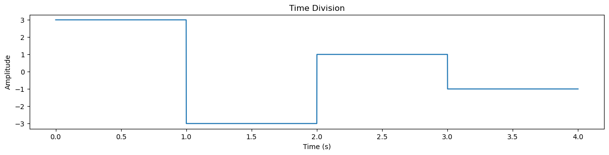
Time Division Transmission

• Method: Divide the total time interval \(T_1\) into 4 equal time slots, each of duration \(T = T_1 / 4\).

• Process: Transmit each component \(s_i\) of the signal vector sequentially in its respective time slot.

  • Time Slot 1: Transmit \(s_1\)

  • Time Slot 2: Transmit \(s_2\)

  • Time Slot 3: Transmit \(s_3\)

  • Time Slot 4: Transmit \(s_4\)

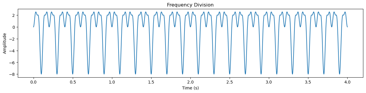
Frequency Division Transmission

• Method: Divide the frequency band into 4 slots, each of width \(\Delta f\), ensuring enough spacing to prevent cross-talk.

• Process: Transmit each component \(s_i\) on a separate frequency carrier:

  • Carrier 1 (Frequency \(f_1\)): Modulate amplitude \(s_1\)

  • Carrier 2 (Frequency \(f_2\)): Modulate amplitude \(s_2\)

  • Carrier 3 (Frequency \(f_3\)): Modulate amplitude \(s_3\)

  • Carrier 4 (Frequency \(f_4\)): Modulate amplitude \(s_4\)

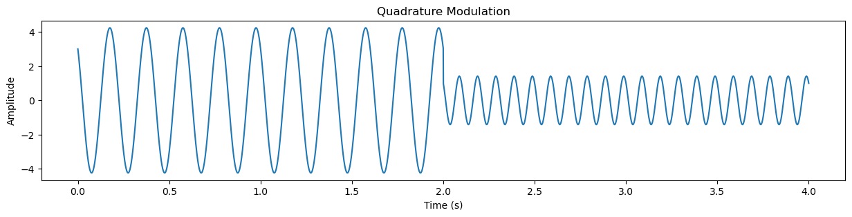
Quadrature Modulation (Using Phase and Amplitude)

• Method: Use quadrature carriers (sinusoidal carriers in phase quadrature) to transmit 2 components of the signal simultaneously in one time slot.

• Process:

  • Time Slot 1:

    • Carrier 1: Transmit \(s_1\) (amplitude modulated on cosine)

    • Carrier 1: Transmit \(s_2\) (amplitude modulated on sine)

  • Time Slot 2:

    • Carrier 2: Transmit \(s_3\) (amplitude modulated on cosine)

    • Carrier 2: Transmit \(s_4\) (amplitude modulated on sine)

Hybrid Time and Frequency Division

• Method: Use both time and frequency resources to transmit the signal efficiently.

• Process: Divide the 4-dimensional signal into 2 pairs:

  • Pair 1: \([s_1, s_2]\)

  • Pair 2: \([s_3, s_4]\)

  Each pair is transmitted in a separate time slot (\(T_1/2\)) over 2 frequency carriers:

  • Time Slot 1:

    • \(f_1\): Transmit \(s_1\)

    • \(f_2\): Transmit \(s_2\)

  • Time Slot 2:

    • \(f_1\): Transmit \(s_3\)

    • \(f_2\): Transmit \(s_4\)

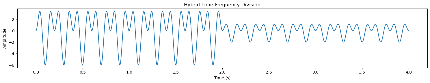
Details on Hybrid Time-Frequency Division Method

In the hybrid time-frequency division method, both time and frequency domains are utilized to efficiently transmit the signal components. Here’s how it works with the example:

Simulation Setup

1. Binary Data:

   • Binary data: \([1, 0, 1, 1, 0, 1, 0, 0]\).

   • Each pair of bits is mapped to one component of the signal vector (\(s_1, s_2, s_3, s_4\)) using Binary PAM:

     • \(00 \rightarrow -3\)

     • \(01 \rightarrow -1\)

     • \(10 \rightarrow +1\)

     • \(11 \rightarrow +3\)

   • Signal vector: \( \vec{s} = [s_1, s_2, s_3, s_4] = [3, -3, 1, -1] \).

2. Waveforms for Components:

   • Each component \(s_i\) corresponds to a rectangular pulse of duration \(T\).

Hybrid Transmission Steps

1. Divide the Signal into Pairs:

   • Split the 4-dimensional signal vector into two pairs:

     • Pair 1: \([s_1, s_2]\)

     • Pair 2: \([s_3, s_4]\)

2. Use Time Slots:

   • Use two time slots (\(T_1\) and \(T_2\)), each of duration \(T\), for the two pairs.

3. Use Frequency Slots:

   • Within each time slot, use two frequency slots (\(f_1\) and \(f_2\)) to transmit the pair of components.

Waveform Example

Time Slot 1:

• Frequency Slot \(f_1\):

  • Transmit \(s_1 = 3\) using a cosine carrier:

    \[ x_{1, f_1}(t) = 3\cos(2\pi f_1 t), \quad 0 \leq t < T \]

• Frequency Slot \(f_2\):

  • Transmit \(s_2 = -3\) using a cosine carrier:

    \[ x_{1, f_2}(t) = -3\cos(2\pi f_2 t), \quad 0 \leq t < T \]

Time Slot 2:

• Frequency Slot \(f_1\):

  • Transmit \(s_3 = 1\) using a cosine carrier:

    \[ x_{2, f_1}(t) = 1\cos(2\pi f_1 t), \quad T \leq t < 2T \]

• Frequency Slot \(f_2\):

  • Transmit \(s_4 = -1\) using a cosine carrier:

    \[ x_{2, f_2}(t) = -1\cos(2\pi f_2 t), \quad T \leq t < 2T \]

Combined Waveform

The total transmitted signal is the sum of the components across the time and frequency slots:

\[\begin{split} x(t) = \begin{cases} 3\cos(2\pi f_1 t) - 3\cos(2\pi f_2 t), & 0 \leq t < T, \\ 1\cos(2\pi f_1 t) - 1\cos(2\pi f_2 t), & T \leq t < 2T \end{cases} \end{split}\]

Resource Allocation

Time Slot	Frequency Slot \(f_1\)	Frequency Slot \(f_2\)
Slot 1	Transmit \(s_1 = 3\)	Transmit \(s_2 = -3\)
Slot 2	Transmit \(s_3 = 1\)	Transmit \(s_4 = -1\)

Comparison with Other Methods

Method	Time Slots	Frequency Slots	Spectral Efficiency	Complexity
Time Division	4	1	Low	Low (simple implementation)
Frequency Division	1	4	Low	Moderate
Quadrature Modulation	2	2	High	High (phase synchronization)
Hybrid (Time-Frequency)	2	2	Moderate	Moderate

import numpy as np
import matplotlib.pyplot as plt

# Simulation parameters
T = 1  # Time slot duration
fs = 1000  # Sampling frequency
t = np.linspace(0, 4*T, 4*fs)  # Total time for the simulation (4 time slots)

# Signal vector components
s = [3, -3, 1, -1]  # s1, s2, s3, s4
frequencies = [5, 10, 15, 20]  # Frequency slots in Hz for frequency division
f1, f2 = 5, 10  # Two carriers for hybrid and quadrature modulation

# Time slots for time division
time_division = np.zeros_like(t)
for i, si in enumerate(s):
    start = int(i * fs)
    end = int((i + 1) * fs)
    time_division[start:end] = si

# Frequency division signals
frequency_division = (
    s[0] * np.cos(2 * np.pi * frequencies[0] * t) +
    s[1] * np.cos(2 * np.pi * frequencies[1] * t) +
    s[2] * np.cos(2 * np.pi * frequencies[2] * t) +
    s[3] * np.cos(2 * np.pi * frequencies[3] * t)
)

# Quadrature modulation signals
quadrature_modulation = (
    (s[0] * np.cos(2 * np.pi * f1 * t) + s[1] * np.sin(2 * np.pi * f1 * t)) *
    (t < 2*T).astype(float) +
    (s[2] * np.cos(2 * np.pi * f2 * t) + s[3] * np.sin(2 * np.pi * f2 * t)) *
    (t >= 2*T).astype(float)
)

# Hybrid time-frequency division signals
hybrid_time_frequency = (
    (s[0] * np.cos(2 * np.pi * f1 * t) + s[1] * np.cos(2 * np.pi * f2 * t)) *
    (t < 2*T).astype(float) +
    (s[2] * np.cos(2 * np.pi * f1 * t) + s[3] * np.cos(2 * np.pi * f2 * t)) *
    (t >= 2*T).astype(float)
)

# Plotting the waveforms

# Time Division
plt.figure(figsize=(15, 3))
plt.plot(t, time_division)
plt.title("Time Division")
plt.xlabel("Time (s)")
plt.ylabel("Amplitude")

# Frequency Division
plt.figure(figsize=(15, 3))
plt.plot(t, frequency_division)
plt.title("Frequency Division")
plt.xlabel("Time (s)")
plt.ylabel("Amplitude")

# Quadrature Modulation
plt.figure(figsize=(15, 3))
plt.plot(t, quadrature_modulation)
plt.title("Quadrature Modulation")
plt.xlabel("Time (s)")
plt.ylabel("Amplitude")

# Hybrid Time-Frequency Division
plt.figure(figsize=(15, 3))
plt.plot(t, hybrid_time_frequency)
plt.title("Hybrid Time-Frequency Division")
plt.xlabel("Time (s)")
plt.ylabel("Amplitude")

plt.tight_layout()
plt.show()

# Compute frequency domain representations
from scipy.fft import fft, fftfreq

def compute_fft(signal, fs):
    N = len(signal)
    yf = fft(signal)
    xf = fftfreq(N, 1/fs)[:N//2]
    return xf, np.abs(yf[:N//2])

# Frequency domain calculations
xf_time, yf_time = compute_fft(time_division, fs)
xf_freq, yf_freq = compute_fft(frequency_division, fs)
xf_quad, yf_quad = compute_fft(quadrature_modulation, fs)
xf_hybrid, yf_hybrid = compute_fft(hybrid_time_frequency, fs)

# Plot frequency domain

# Time Division
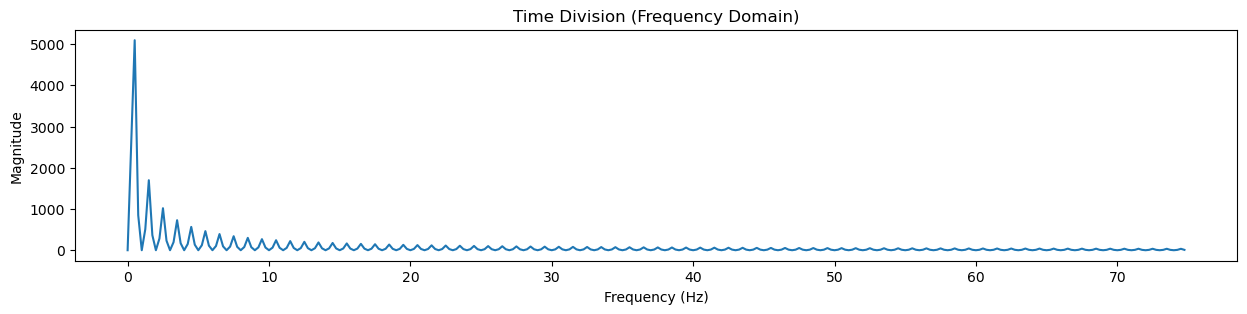
plt.figure(figsize=(15, 3))
plt.plot(xf_time[:300], yf_time[:300])
plt.title("Time Division (Frequency Domain)")
plt.xlabel("Frequency (Hz)")
plt.ylabel("Magnitude")

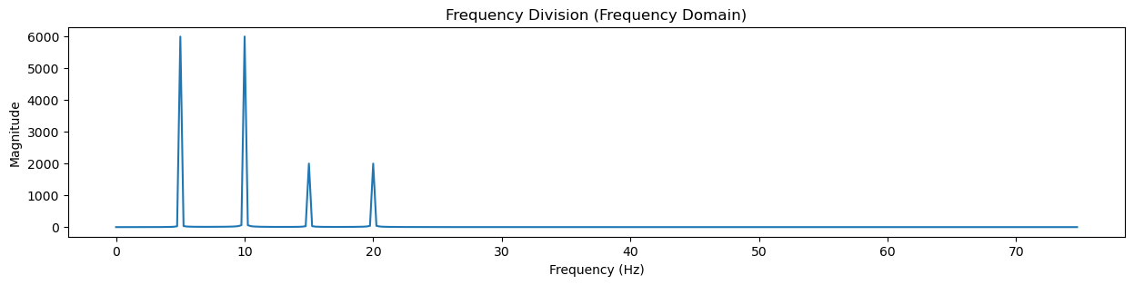
# Frequency Division
plt.figure(figsize=(15, 3))
plt.plot(xf_freq[:300], yf_freq[:300])
plt.title("Frequency Division (Frequency Domain)")
plt.xlabel("Frequency (Hz)")
plt.ylabel("Magnitude")

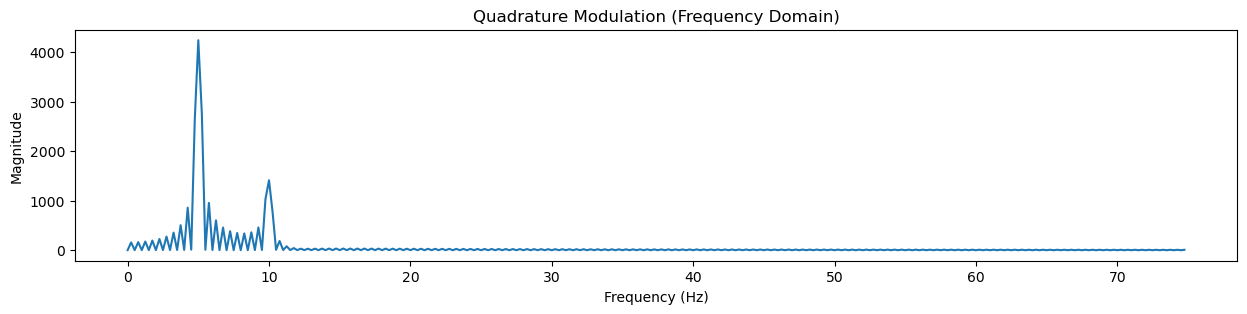
# Quadrature Modulation
plt.figure(figsize=(15, 3))
plt.plot(xf_quad[:300], yf_quad[:300])
plt.title("Quadrature Modulation (Frequency Domain)")
plt.xlabel("Frequency (Hz)")
plt.ylabel("Magnitude")

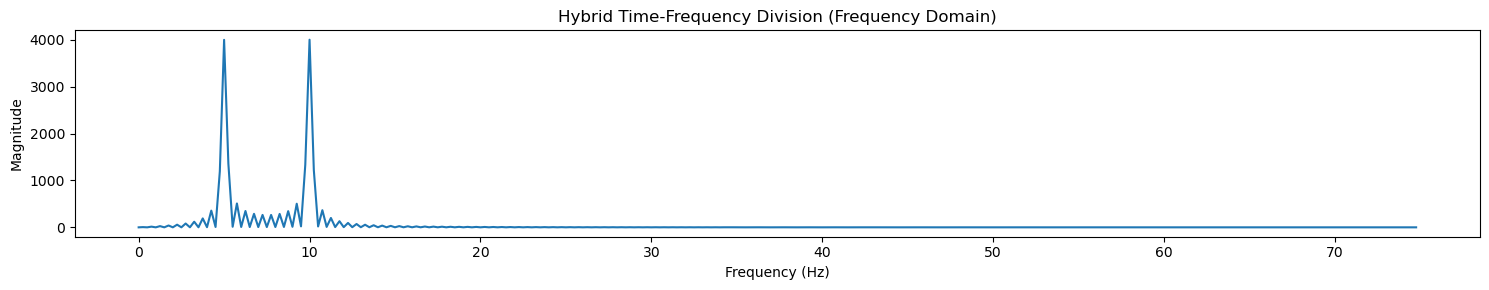
# Hybrid Time-Frequency Division
plt.figure(figsize=(15, 3))
plt.plot(xf_hybrid[:300], yf_hybrid[:300])
plt.title("Hybrid Time-Frequency Division (Frequency Domain)")
plt.xlabel("Frequency (Hz)")
plt.ylabel("Magnitude")

plt.tight_layout()
plt.show()