Lossless Data Compression Algorithms#
The Huffman Coding Algorithm#
In 1952, David Albert Huffman developed the Huffman Coding Algorithm, a variable-length encoding method that constructs an optimal code based on the probabilities of source symbols, \( P(x_i) \) for \( i = 1, 2, \dots, L \).
This algorithm minimizes the average number of binary digits (bits) required to represent the symbols of a discrete memoryless source (DMS), while adhering to the prefix condition—ensuring that no code word is a prefix of another, making the code uniquely and instantaneously decodable.
Huffman coding achieves efficiency by assigning shorter code words to more probable symbols and longer ones to less probable symbols, aligning with the entropy bounds described by Shannon’s first theorem.
Optimality and Decodability#
Huffman coding is optimal in the sense that it produces the smallest possible average code word length, \( \bar{R} \), among all prefix codes for a given source, typically approaching the source entropy, \( H(X) \), within 1 bit:
The prefix condition ensures that the received bit sequence can be decoded instantly—each code word is recognized as soon as its last bit is received, eliminating ambiguity and delay. This property makes Huffman coding both theoretically significant and practically valuable for applications such as file compression (e.g., ZIP) and data transmission.
Example 1: Huffman Coding and Alternative Code#
Source Description and Initial Setup#
Consider a discrete memoryless source (DMS) with seven symbols:
The symbols are arranged in decreasing order of probability:
The assigned probabilities are:
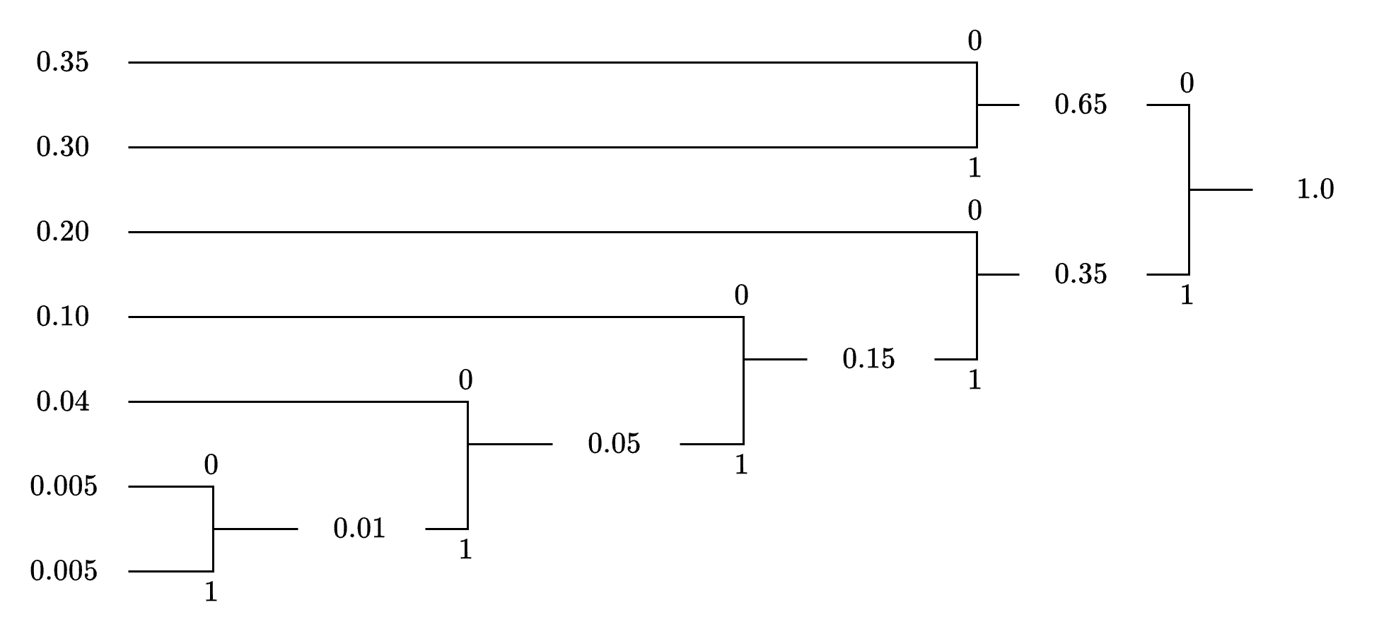
The Huffman algorithm constructs a binary tree by iteratively combining the two least probable symbols, assigning bits (0 or 1) to branches, and forming code words from the tree structure. The process begins with the two least probable symbols, \( x_6 \) and \( x_7 \), both having probability 0.005.
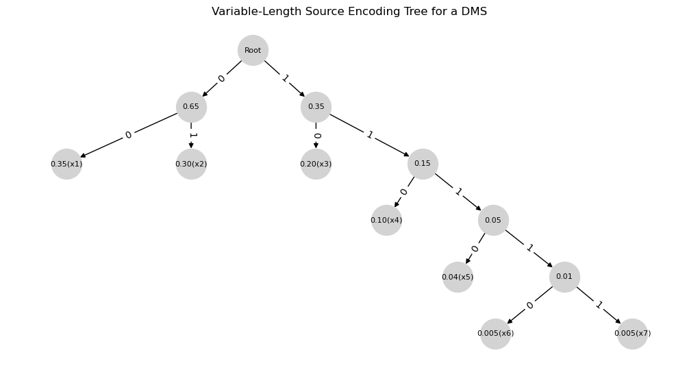
 Variable-Length Source Encoding Tree for a DMS
import matplotlib.pyplot as plt
import networkx as nx

# Create a directed graph
G = nx.DiGraph()

# Define the tree structure with probabilities
edges = [
    ("Root", "0.65", 0), ("Root", "0.35", 1),
    ("0.65", "0.35(x1)", 0), ("0.65", "0.30(x2)", 1),
    ("0.35", "0.20(x3)", 0), ("0.35", "0.15", 1),
    ("0.15", "0.10(x4)", 0), ("0.15", "0.05", 1),
    ("0.05", "0.04(x5)", 0), ("0.05", "0.01", 1),
    ("0.01", "0.005(x6)", 0), ("0.01", "0.005(x7)", 1)
]

# Add nodes and edges
for parent, child, label in edges:
    G.add_edge(parent, child, label=label)

# Positioning the nodes
pos = nx.drawing.nx_agraph.graphviz_layout(G, prog="dot")

# Draw the graph
plt.figure(figsize=(10, 5))
nx.draw(G, pos, with_labels=True, node_size=1000, node_color="lightgray", edge_color="black", font_size=8)

# Draw edge labels
edge_labels = {(parent, child): label for parent, child, label in edges}
nx.draw_networkx_edge_labels(G, pos, edge_labels=edge_labels, font_size=10)

# Show the diagram
plt.title("Variable-Length Source Encoding Tree for a DMS")
plt.show()
Code Tree Construction#
The first step in the Huffman tree construction involves merging \( x_6 \) and \( x_7 \) into a single node with probability:
We assign 0 to the upper branch (e.g., \( x_6 \)) and 1 to the lower branch (e.g., \( x_7 \)).
This new node, with probability 0.01, is treated as a new symbol in the next iteration.
The process continues by repeatedly merging the two symbols or nodes with the lowest probabilities, building the tree bottom-up.
Full Tree Construction and Code Words#
The Huffman tree is built iteratively by merging the two least probable symbols at each step:
First Merge: Combine the node (0.01) with \( x_5 \) (0.04): \( 0.01 + 0.04 = 0.05 \)
Second Merge: Combine (0.05) with \( x_4 \) (0.10): \( 0.05 + 0.10 = 0.15 \)
Third Merge: Combine (0.15) with \( x_3 \) (0.20): \( 0.15 + 0.20 = 0.35 \)
Fourth Merge: Combine (0.35) with \( x_2 \) (0.30): \( 0.35 + 0.30 = 0.65 \)
Final Merge: Combine (0.65) with \( x_1 \) (0.35): \( 0.65 + 0.35 = 1.0 \)
Code Words (Read from Root to Leaf):
\( x_1 \): 00 (Root → 0.65 → 0.35)
\( x_2 \): 01 (Root → 0.65 → 0.30)
\( x_3 \): 10 (Root → 0.35 → 0.20)
\( x_4 \): 110 (Root → 0.35 → 0.15 → 0.10)
\( x_5 \): 1110 (Root → 0.35 → 0.15 → 0.05 → 0.04)
\( x_6 \): 11110 (Root → 0.35 → 0.15 → 0.05 → 0.01 → 0.005(x6))
\( x_7 \): 11111 (Root → 0.35 → 0.15 → 0.05 → 0.01 → 0.005(x7))
class Node:
    def __init__(self, symbol, probability):
        self.symbol = symbol
        self.probability = probability
        self.code = ""
        self.left = None
        self.right = None

# Constructing the probability tree based on given edges
def build_tree():
    nodes = {
        "0.65": Node("", 0.65),
        "0.35": Node("", 0.35),
        "0.35(x1)": Node("x1", 0.35),
        "0.30(x2)": Node("x2", 0.30),
        "0.20(x3)": Node("x3", 0.20),
        "0.15": Node("", 0.15),
        "0.10(x4)": Node("x4", 0.10),
        "0.05": Node("", 0.05),
        "0.04(x5)": Node("x5", 0.04),
        "0.01": Node("", 0.01),
        "0.005(x6)": Node("x6", 0.005),
        "0.005(x7)": Node("x7", 0.005)
    }

    edges = [
        ("Root", "0.65", 0), ("Root", "0.35", 1),
        ("0.65", "0.35(x1)", 0), ("0.65", "0.30(x2)", 1),
        ("0.35", "0.20(x3)", 0), ("0.35", "0.15", 1),
        ("0.15", "0.10(x4)", 0), ("0.15", "0.05", 1),
        ("0.05", "0.04(x5)", 0), ("0.05", "0.01", 1),
        ("0.01", "0.005(x6)", 0), ("0.01", "0.005(x7)", 1)
    ]

    root = Node("Root", 1.0)
    root.left = nodes["0.65"]
    root.right = nodes["0.35"]

    for parent, child, bit in edges:
        if parent == "Root":
            parent_node = root
        else:
            parent_node = nodes[parent]

        child_node = nodes[child]
        child_node.code = parent_node.code + str(bit)

        if bit == 0:
            parent_node.left = child_node
        else:
            parent_node.right = child_node

    return root

# Extract the symbol codes from the tree
def extract_codes(node, codes):
    if node is None:
        return
    if node.symbol:
        codes[node.symbol] = node.code
    extract_codes(node.left, codes)
    extract_codes(node.right, codes)

# Main execution
if __name__ == "__main__":
    root = build_tree()
    codes = {}
    extract_codes(root, codes)

    print("Variable-Length Encoding:")
    for symbol, code in sorted(codes.items(), key=lambda x: x[1]):
        print(f"{symbol}: {code}")
Variable-Length Encoding:
Root:
x1: 00
x2: 01
x3: 10
x4: 110
x5: 1110
x6: 11110
x7: 11111
Entropy and Average Length Calculation#
Entropy Calculation (Base 2):#
Expanding the terms:
Average Code Length Calculation:#
Since Huffman coding follows the source coding theorem, we verify:
Thus, the Huffman code is efficient, achieving an average length close to the source entropy.
Letter |
Probability |
Self-information |
Code |
|---|---|---|---|
\( x_1 \) |
0.35 |
1.5146 |
00 |
\( x_2 \) |
0.30 |
1.7370 |
01 |
\( x_3 \) |
0.20 |
2.3219 |
10 |
\( x_4 \) |
0.10 |
3.3219 |
110 |
\( x_5 \) |
0.04 |
4.6439 |
1110 |
\( x_6 \) |
0.005 |
7.6439 |
11110 |
\( x_7 \) |
0.005 |
7.6439 |
11111 |
Entropy: \( H(X) = 2.11 \)
Average code length: \( \bar{R} = 2.21 \)
import numpy as np

def compute_self_information(probabilities):
    return -np.log2(probabilities)

def compute_entropy(probabilities):
    return -np.sum(probabilities * np.log2(probabilities))

# Probabilities for each letter in the code X
probabilities_code = np.array([0.35, 0.30, 0.20, 0.10, 0.04, 0.005, 0.005])

# Compute self-information for each component
self_information = compute_self_information(probabilities_code)

# Calculate the entropy of X
entropy_X = compute_entropy(probabilities_code)

# Print self-information
print("Self-information:")
for value in self_information:
    print(f"{value:.4f}")

# Print entropy
print(f"Entropy: {entropy_X:.2f}")

# Using Tables provided above
# Lengths of the code words for each letter
code_lengths = np.array([2, 2, 2, 3, 4, 5, 5])

# Calculate R_bar for the code X
R_bar = np.sum(probabilities_code * code_lengths)
print(f"Average Code Length: {R_bar:.2f}")

# Using alternative Tables provided below
# Updated code lengths
code_lengths_new = np.array([1, 2, 3, 4, 5, 6, 6])

# Recalculate R_bar for the updated lengths
R_bar_new = np.sum(probabilities_code * code_lengths_new)
print(f"Average Code Length (new): {R_bar_new:.2f}")

# Encoding and Decoding Functions
def encode_given_code(sequence, codebook):
    """Encodes a sequence of letters based on the given codebook."""
    return ''.join(codebook[letter] for letter in sequence)

def decode_given_code(encoded_sequence, codebook):
    """Decodes an encoded sequence based on the given codebook."""
    reverse_codebook = {v: k for k, v in codebook.items()}
    decoded_sequence = []
    buffer = ''

    for char in encoded_sequence:
        buffer += char
        if buffer in reverse_codebook:
            decoded_sequence.append(reverse_codebook[buffer])
            buffer = ''

    return decoded_sequence

# Example usage
codebook_given = {
    'x1': '00', 'x2': '01', 'x3': '10', 'x4': '110', 'x5': '1110', 'x6': '11110', 'x7': '11111'
}

sequence_to_encode = ['x1', 'x3', 'x4', 'x5', 'x7']
encoded_sequence = encode_given_code(sequence_to_encode, codebook_given)
decoded_sequence = decode_given_code(encoded_sequence, codebook_given)

print("Encoded Sequence:", encoded_sequence)
print("Decoded Sequence:", ' '.join(decoded_sequence))
Self-information:
1.5146
1.7370
2.3219
3.3219
4.6439
7.6439
7.6439
Entropy: 2.11
Average Code Length: 2.21
Average Code Length (new): 2.21
Encoded Sequence: 0010110111011111
Decoded Sequence: x1 x3 x4 x5 x7
Non-Uniqueness of Huffman Codes#
Huffman codes are not necessarily unique, as different choices during tree construction (e.g., selecting which pairs to merge when probabilities are equal) can result in distinct codes with the same average code length \( \bar{R} \).
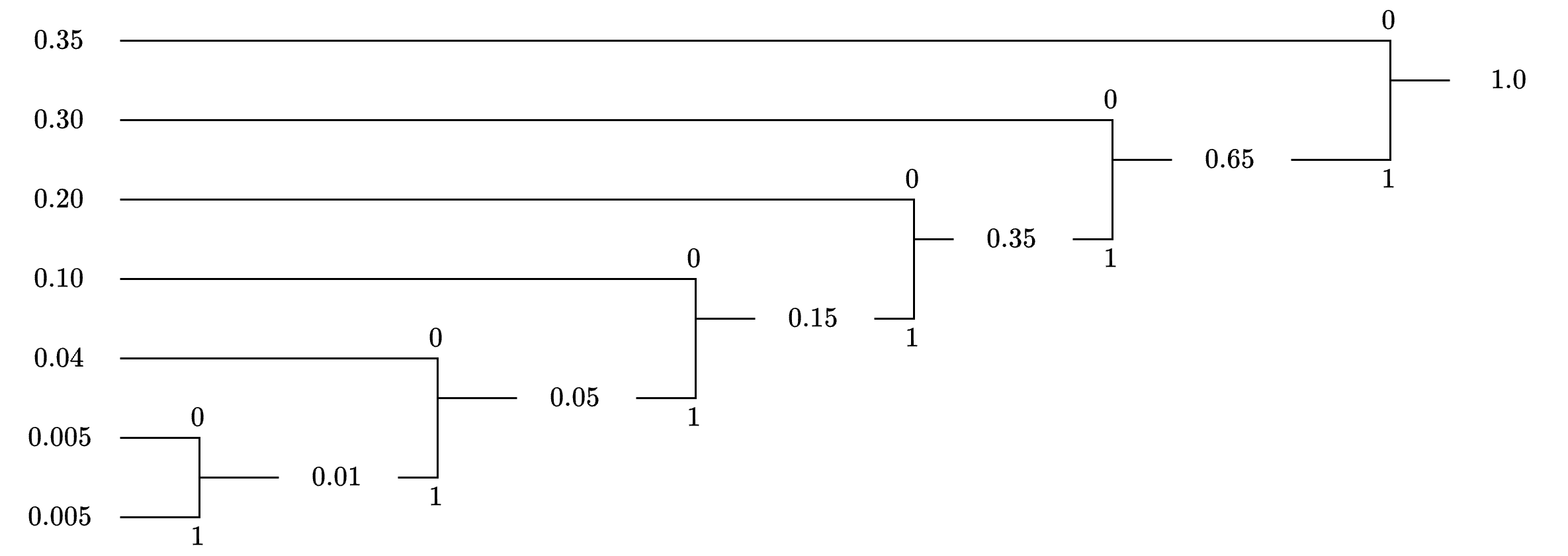
In our example, at the step where two nodes of probability 0.35 exist—one from \( x_1 \) and another from previous merges—we paired \( x_1 \) with \( x_2 \). However, an alternative approach would be to pair \( x_2 \) with the 0.35 node containing \( x_3 \), leading to a different Huffman tree.
Alternative Huffman Code#
Using an alternative pairing order, the tree construction follows these steps:
Merge \( x_6 \) and \( x_7 \): \( 0.005 + 0.005 = 0.01 \)
Merge \( (0.01) \) and \( x_5 \): \( 0.01 + 0.04 = 0.05 \)
Merge \( (0.05) \) and \( x_4 \): \( 0.05 + 0.10 = 0.15 \)
Merge \( (0.15) \) and \( x_3 \): \( 0.15 + 0.20 = 0.35 \)
Merge \( (0.35) \) and \( x_2 \): \( 0.35 + 0.30 = 0.65 \)
Final Merge \( (0.65) \) and \( x_1 \): \( 0.65 + 0.35 = 1.0 \)
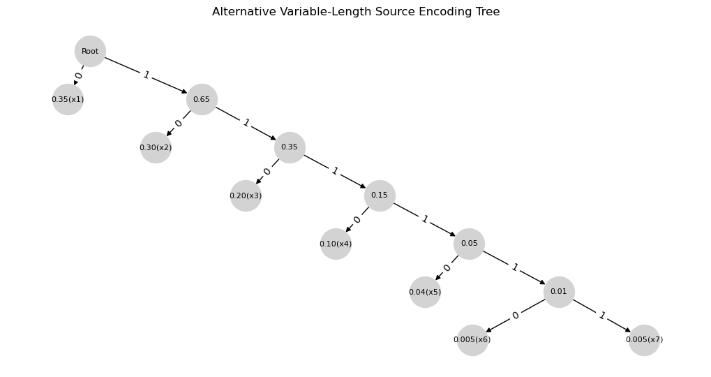
Code Words for the Alternative Tree:
\( x_1 \): 0
\( x_2 \): 10
\( x_3 \): 110
\( x_4 \): 1110
\( x_5 \): 11110
\( x_6 \): 111110
\( x_7 \): 111111
 Alternative Variable-Length Source Encoding Tree
# Create a new directed graph for the alternative tree
G_alt = nx.DiGraph()

# Define the alternative tree structure with probabilities
edges_alt = [
    ("Root", "0.35(x1)", 0), ("Root", "0.65", 1),
    ("0.65", "0.30(x2)", 0), ("0.65", "0.35", 1),
    ("0.35", "0.20(x3)", 0), ("0.35", "0.15", 1),
    ("0.15", "0.10(x4)", 0), ("0.15", "0.05", 1),
    ("0.05", "0.04(x5)", 0), ("0.05", "0.01", 1),
    ("0.01", "0.005(x6)", 0), ("0.01", "0.005(x7)", 1)
]

# Add nodes and edges for the alternative tree
for parent, child, label in edges_alt:
    G_alt.add_edge(parent, child, label=label)

# Positioning the nodes for the alternative tree
pos_alt = nx.drawing.nx_agraph.graphviz_layout(G_alt, prog="dot")

# Draw the alternative tree graph
plt.figure(figsize=(10, 5))
nx.draw(G_alt, pos_alt, with_labels=True, node_size=1000, node_color="lightgray", edge_color="black", font_size=8)

# Draw edge labels for the alternative tree
edge_labels_alt = {(parent, child): label for parent, child, label in edges_alt}
nx.draw_networkx_edge_labels(G_alt, pos_alt, edge_labels=edge_labels_alt, font_size=10)

# Show the diagram
plt.title("Alternative Variable-Length Source Encoding Tree")
plt.show()
class Node:
    def __init__(self, symbol, probability):
        self.symbol = symbol
        self.probability = probability
        self.code = ""
        self.left = None
        self.right = None

# Constructing the probability tree based on given edges
def build_tree():
    nodes = {
        "0.35(x1)": Node("x1", 0.35),
        "0.65": Node("", 0.65),
        "0.30(x2)": Node("x2", 0.30),
        "0.35": Node("", 0.35),
        "0.20(x3)": Node("x3", 0.20),
        "0.15": Node("", 0.15),
        "0.10(x4)": Node("x4", 0.10),
        "0.05": Node("", 0.05),
        "0.04(x5)": Node("x5", 0.04),
        "0.01": Node("", 0.01),
        "0.005(x6)": Node("x6", 0.005),
        "0.005(x7)": Node("x7", 0.005)
    }

    edges = [
        ("Root", "0.35(x1)", 0), ("Root", "0.65", 1),
        ("0.65", "0.30(x2)", 0), ("0.65", "0.35", 1),
        ("0.35", "0.20(x3)", 0), ("0.35", "0.15", 1),
        ("0.15", "0.10(x4)", 0), ("0.15", "0.05", 1),
        ("0.05", "0.04(x5)", 0), ("0.05", "0.01", 1),
        ("0.01", "0.005(x6)", 0), ("0.01", "0.005(x7)", 1)
    ]

    root = Node("Root", 1.0)
    root.left = nodes["0.35(x1)"]
    root.right = nodes["0.65"]

    for parent, child, bit in edges:
        if parent == "Root":
            parent_node = root
        else:
            parent_node = nodes[parent]

        child_node = nodes[child]
        child_node.code = parent_node.code + str(bit)

        if bit == 0:
            parent_node.left = child_node
        else:
            parent_node.right = child_node

    return root

# Extract the symbol codes from the tree
def extract_codes(node, codes):
    if node is None:
        return
    if node.symbol:
        codes[node.symbol] = node.code
    extract_codes(node.left, codes)
    extract_codes(node.right, codes)

# Main execution
if __name__ == "__main__":
    root = build_tree()
    codes = {}
    extract_codes(root, codes)

    print("Variable-Length Encoding:")
    for symbol, code in sorted(codes.items(), key=lambda x: x[1]):
        print(f"{symbol}: {code}")
Variable-Length Encoding:
Root:
x1: 0
x2: 10
x3: 110
x4: 1110
x5: 11110
x6: 111110
x7: 111111
The average code word length for this alternative tree is computed as:
Breaking it down:
Since both Huffman codes yield \( \bar{R} = 2.21 \), this confirms their equal efficiency despite different structures.
Alternative Code
Letter |
Code |
|---|---|
\( x_1 \) |
0 |
\( x_2 \) |
10 |
\( x_3 \) |
110 |
\( x_4 \) |
1110 |
\( x_5 \) |
11110 |
\( x_6 \) |
111110 |
\( x_7 \) |
111111 |
Average code length: \( \bar{R} = 2.21 \)
Flexibility in Bit Assignment#
The assignment of 0 and 1 to branches is arbitrary. Swapping these assignments (e.g., assigning 1 to the upper branch and 0 to the lower branch) produces another valid prefix code with the same \( \bar{R} \).
For example, reversing the bit assignments in the first code results in:
\( x_1: 11 \)
\( x_2: 10 \)
\( x_3: 01 \)
\( x_4: 000 \)
\( x_5: 0010 \)
\( x_6: 00110 \)
\( x_7: 00111 \)
This new encoding still satisfies the prefix condition and maintains \( \bar{R} = 2.21 \).
Example 2: Huffman Coding for a DMS#
Source Description and Huffman Tree Structure#
Consider a discrete memoryless source (DMS) with eight symbols:
The assigned probabilities are:
The sum confirms a valid probability distribution:
The Huffman tree is constructed bottom-up by iteratively merging the least probable symbols.
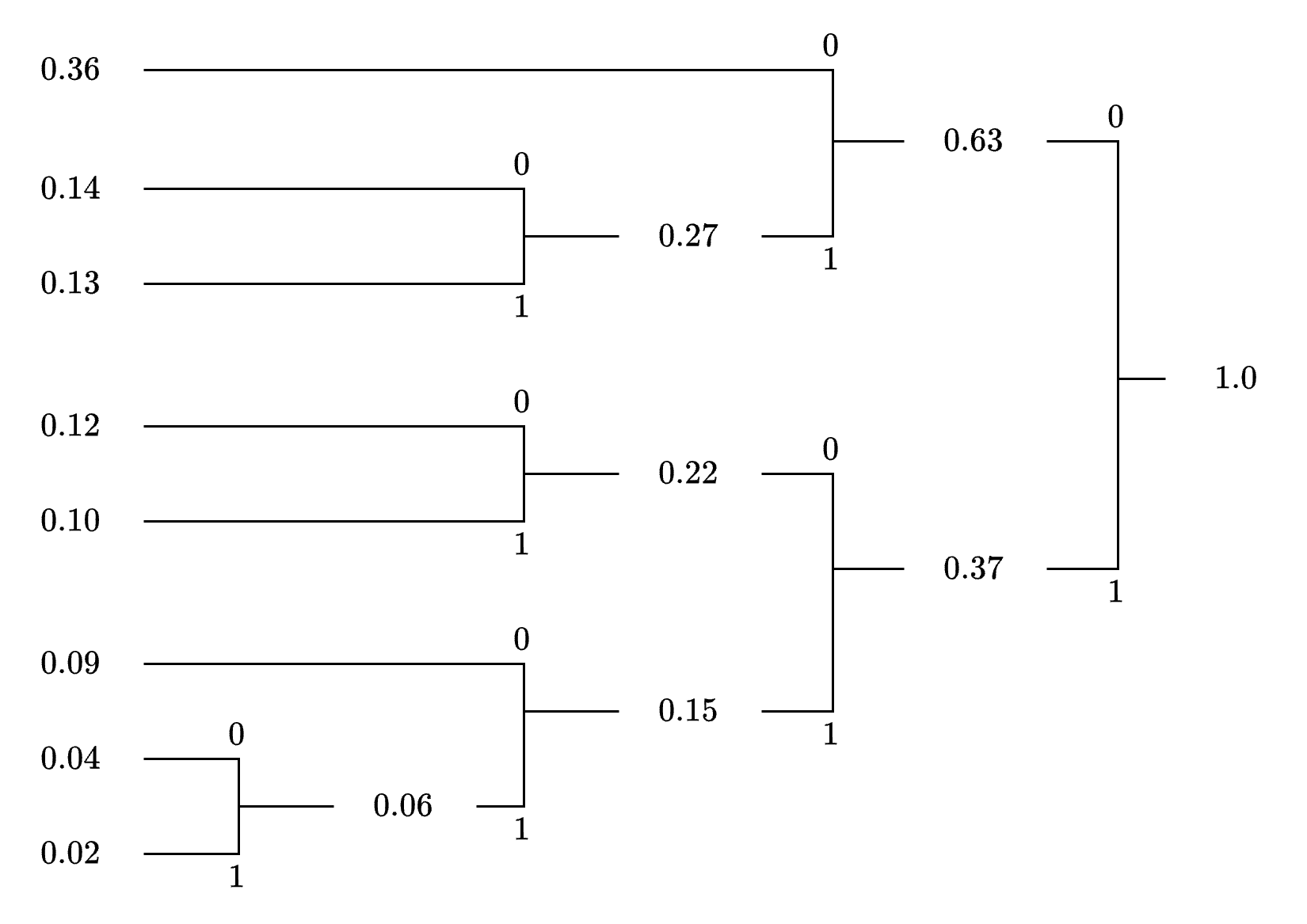 Huffman Coding Tree for DMS
Huffman Code Construction for DMS#
The Huffman algorithm proceeds as follows:
Merge \( x_7 \) and \( x_8 \): \( 0.04 + 0.02 = 0.06 \)
Merge \( (0.06) \) and \( x_6 \): \( 0.06 + 0.09 = 0.15 \)
Merge \( x_5 \) and \( x_4 \): \( 0.10 + 0.12 = 0.22 \)
Merge \( (0.15) \) and \( (0.22) \): \( 0.15 + 0.22 = 0.37 \)
Merge \( x_3 \) and \( x_2 \): \( 0.13 + 0.14 = 0.27 \)
Merge \( (0.27) \) and \( x_1 \): \( 0.27 + 0.36 = 0.63 \)
Final Merge \( (0.63) \) and \( (0.37) \): \( 0.63 + 0.37 = 1.0 \)
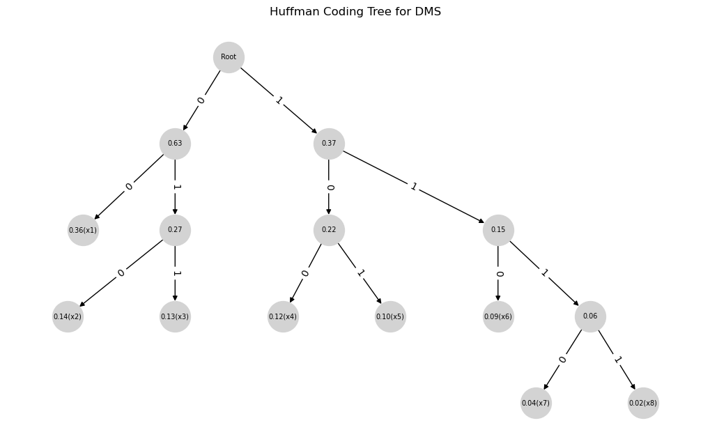
Resulting Code Words (Read from Root to Leaf):
\( x_1 \): 00 (Root → 0.63 → 0.36)
\( x_2 \): 010 (Root → 0.63 → 0.27 → 0.14)
\( x_3 \): 011 (Root → 0.63 → 0.27 → 0.13)
\( x_4 \): 100 (Root → 0.37 → 0.22 → 0.12)
\( x_5 \): 101 (Root → 0.37 → 0.22 → 0.10)
\( x_6 \): 110 (Root → 0.37 → 0.15 → 0.09)
\( x_7 \): 1110 (Root → 0.37 → 0.15 → 0.06 → 0.04)
\( x_8 \): 1111 (Root → 0.37 → 0.15 → 0.06 → 0.02)
Since no code word is a prefix of another, the prefix condition is satisfied.
# Create a new directed graph for the Huffman tree
G_huffman = nx.DiGraph()

# Define the Huffman tree structure with probabilities
edges_huffman = [
    ("Root", "0.63", 0), ("Root", "0.37", 1),
    ("0.63", "0.36(x1)", 0), ("0.63", "0.27", 1),
    ("0.27", "0.14(x2)", 0), ("0.27", "0.13(x3)", 1),
    ("0.37", "0.22", 0), ("0.37", "0.15", 1),
    ("0.22", "0.12(x4)", 0), ("0.22", "0.10(x5)", 1),
    ("0.15", "0.09(x6)", 0), ("0.15", "0.06", 1),
    ("0.06", "0.04(x7)", 0), ("0.06", "0.02(x8)", 1)
]

# Add nodes and edges for the Huffman tree
for parent, child, label in edges_huffman:
    G_huffman.add_edge(parent, child, label=label)

# Positioning the nodes for the Huffman tree
pos_huffman = nx.drawing.nx_agraph.graphviz_layout(G_huffman, prog="dot")

# Draw the Huffman tree graph
plt.figure(figsize=(10, 6))
nx.draw(G_huffman, pos_huffman, with_labels=True, node_size=1000, node_color="lightgray", edge_color="black", font_size=7)

# Draw edge labels for the Huffman tree
edge_labels_huffman = {(parent, child): label for parent, child, label in edges_huffman}
nx.draw_networkx_edge_labels(G_huffman, pos_huffman, edge_labels=edge_labels_huffman, font_size=10)

# Show the diagram
plt.title("Huffman Coding Tree for DMS")
plt.show()
class Node:
    def __init__(self, symbol, probability):
        self.symbol = symbol
        self.probability = probability
        self.code = ""
        self.left = None
        self.right = None

# Constructing the probability tree based on given Huffman edges
def build_tree():
    nodes = {
        "0.63": Node("", 0.63),
        "0.37": Node("", 0.37),
        "0.36(x1)": Node("x1", 0.36),
        "0.27": Node("", 0.27),
        "0.14(x2)": Node("x2", 0.14),
        "0.13(x3)": Node("x3", 0.13),
        "0.22": Node("", 0.22),
        "0.15": Node("", 0.15),
        "0.12(x4)": Node("x4", 0.12),
        "0.10(x5)": Node("x5", 0.10),
        "0.09(x6)": Node("x6", 0.09),
        "0.06": Node("", 0.06),
        "0.04(x7)": Node("x7", 0.04),
        "0.02(x8)": Node("x8", 0.02)
    }

    edges = [
        ("Root", "0.63", 0), ("Root", "0.37", 1),
        ("0.63", "0.36(x1)", 0), ("0.63", "0.27", 1),
        ("0.27", "0.14(x2)", 0), ("0.27", "0.13(x3)", 1),
        ("0.37", "0.22", 0), ("0.37", "0.15", 1),
        ("0.22", "0.12(x4)", 0), ("0.22", "0.10(x5)", 1),
        ("0.15", "0.09(x6)", 0), ("0.15", "0.06", 1),
        ("0.06", "0.04(x7)", 0), ("0.06", "0.02(x8)", 1)
    ]

    root = Node("Root", 1.0)
    root.left = nodes["0.63"]
    root.right = nodes["0.37"]

    for parent, child, bit in edges:
        if parent == "Root":
            parent_node = root
        else:
            parent_node = nodes[parent]

        child_node = nodes[child]
        child_node.code = parent_node.code + str(bit)

        if bit == 0:
            parent_node.left = child_node
        else:
            parent_node.right = child_node

    return root

# Extract the symbol codes from the tree
def extract_codes(node, codes):
    if node is None:
        return
    if node.symbol:
        codes[node.symbol] = node.code
    extract_codes(node.left, codes)
    extract_codes(node.right, codes)

# Main execution
if __name__ == "__main__":
    root = build_tree()
    codes = {}
    extract_codes(root, codes)

    print("Variable-Length Huffman Encoding:")
    for symbol, code in sorted(codes.items(), key=lambda x: x[1]):
        print(f"{symbol}: {code}")
Variable-Length Huffman Encoding:
Root:
x1: 00
x2: 010
x3: 011
x4: 100
x5: 101
x6: 110
x7: 1110
x8: 1111
Entropy Calculation#
The entropy \( H(X) \) of the source (base 2) is:
Expanding the terms:
Average Code Word Length Calculation#
The average code word length \( \bar{R} \) is given by:
where \( n_i \) is the length of each Huffman code word:
\( x_1 \): (00) → 2 bits, \( 0.36 \times 2 = 0.72 \)
\( x_2 \): (010) → 3 bits, \( 0.14 \times 3 = 0.42 \)
\( x_3 \): (011) → 3 bits, \( 0.13 \times 3 = 0.39 \)
\( x_4 \): (100) → 3 bits, \( 0.12 \times 3 = 0.36 \)
\( x_5 \): (101) → 3 bits, \( 0.10 \times 3 = 0.30 \)
\( x_6 \): (110) → 3 bits, \( 0.09 \times 3 = 0.27 \)
\( x_7 \): (1110) → 4 bits, \( 0.04 \times 4 = 0.16 \)
\( x_8 \): (1111) → 4 bits, \( 0.02 \times 4 = 0.08 \)
Summing these values:
Coding Efficiency#
The coding efficiency \( \eta \) is computed as:
Rounded to two decimal places:
This means the Huffman code operates at 97% efficiency, reflecting its near-optimality since \( \bar{R} \) is very close to \( H(X) \).
Verification of the Source Coding Theorem#
The Source Coding Theorem for prefix codes states:
Substituting the values:
Since this inequality holds, the Huffman code satisfies the theoretical bound, confirming its validity and alignment with information theory principles.
Letter |
Code |
|---|---|
\( x_1 \) |
00 |
\( x_2 \) |
010 |
\( x_3 \) |
011 |
\( x_4 \) |
100 |
\( x_5 \) |
101 |
\( x_6 \) |
110 |
\( x_7 \) |
1110 |
\( x_8 \) |
1111 |
Entropy: \( H(X) = 2.62 \)
Average code length: \( \bar{R} = 2.70 \)
Encoding Blocks of Symbols#
Block Encoding for Efficiency#
Instead of encoding a discrete memoryless source (DMS) symbol-by-symbol, greater efficiency can be achieved by encoding blocks of \( J \) symbols at a time.
For a DMS, the entropy of a \( J \)-symbol block is:
Since the symbols are independent, the joint entropy is additive. The average number of bits per block for a Huffman code applied to these blocks satisfies:
This extends the source coding theorem for prefix codes from single-symbol encoding to block encoding. Dividing by \( J \), the average bits per symbol becomes:
where:
is the per-symbol rate. As \( J \) increases, the term \( \frac{1}{J} \) shrinks, allowing \( \bar{R} \) to approach \( H(X) \) arbitrarily closely, thus improving compression efficiency compared to single-symbol encoding.
Intuition and Advantage
Symbol-by-symbol encoding often results in \( \bar{R} \) exceeding \( H(X) \) by a fraction of a bit due to the integer constraint on code word lengths.
Block encoding amortizes this overhead across \( J \) symbols, reducing the per-symbol excess to:
thus nearing the entropy limit—a key insight for practical compression systems.
Example 3: Single Symbol Encoding#
Source Description
Consider a DMS with three symbols:
with probabilities:
Entropy Calculation
The entropy \( H(X) \) (base 2) is:
Expanding each term:
\( P(x_1) = 0.45 \), \( \log_2 0.45 \approx 1.1520 \), \( -0.45 \times 1.1520 = -0.5184 \)
\( P(x_2) = 0.35 \), \( \log_2 0.35 \approx 1.5146 \), \( -0.35 \times 1.5146 = -0.5301 \)
\( P(x_3) = 0.20 \), \( \log_2 0.20 \approx 2.3219 \), \( -0.20 \times 2.3219 = -0.4644 \)
Summing:
Huffman Code and Average Length#
The Huffman code for single symbols is:
\( x_1 \) : (1) → 1 bit
\( x_2 \) : (00) → 2 bits
\( x_3 \) : (01) → 2 bits
Average Code Length Calculation:#
Bounds Verification:
This satisfies the source coding theorem:
Efficiency Calculation#
The coding efficiency \( \eta \) is:
Rounded to two decimal places:
The excess:
reflects the integer-length constraint on Huffman code words, resulting in high but not perfect efficiency.
Table: Huffman code for Example 3#
Letter |
Probability |
Self-information |
Code |
|---|---|---|---|
\( x_1 \) |
0.45 |
1.156 |
1 |
\( x_2 \) |
0.35 |
1.520 |
00 |
\( x_3 \) |
0.20 |
2.330 |
01 |
Additional information:
\( H(X) = 1.513 \) bits/letter
\( \bar{R_1} = 1.55 \) bits/letter
Efficiency = 97.6%
Example 3 (continued) - Encoding Pairs of Symbols#
Block Encoding Setup#
For \( J = 2 \), we encode pairs of symbols. Since the source is memoryless, the joint probability of two symbols appearing together is:
The probabilities for all symbol pairs are:
\( x_1 x_1 \): \( 0.45 \times 0.45 = 0.2025 \)
\( x_1 x_2 \): \( 0.45 \times 0.35 = 0.1575 \)
\( x_2 x_1 \): \( 0.35 \times 0.45 = 0.1575 \)
\( x_2 x_2 \): \( 0.35 \times 0.35 = 0.1225 \)
\( x_1 x_3 \): \( 0.45 \times 0.20 = 0.09 \)
\( x_3 x_1 \): \( 0.20 \times 0.45 = 0.09 \)
\( x_2 x_3 \): \( 0.35 \times 0.20 = 0.07 \)
\( x_3 x_2 \): \( 0.20 \times 0.35 = 0.07 \)
\( x_3 x_3 \): \( 0.20 \times 0.20 = 0.04 \)
Summing:
confirming a valid probability distribution.
Entropy of Pairs#
The joint entropy for symbol pairs is:
Table: Huffman Code for Encoding Pairs of Letters
Letter Pair |
Probability |
Self-information |
Code |
|---|---|---|---|
\( x_1 x_1 \) |
0.2025 |
2.312 |
10 |
\( x_1 x_2 \) |
0.1575 |
2.676 |
001 |
\( x_2 x_1 \) |
0.1575 |
2.676 |
010 |
\( x_2 x_2 \) |
0.1225 |
3.039 |
011 |
\( x_1 x_3 \) |
0.09 |
3.486 |
111 |
\( x_3 x_1 \) |
0.09 |
3.486 |
0000 |
\( x_2 x_3 \) |
0.07 |
3.850 |
0001 |
\( x_3 x_2 \) |
0.07 |
3.850 |
1100 |
\( x_3 x_3 \) |
0.04 |
4.660 |
1101 |
Additional information:
\( 2H(X) = 3.026 \) bits/letter pair
\( \bar{R_2} = 3.0675 \) bits/letter pair
\( \frac{1}{2} \bar{R_2} = 1.534 \) bits/letter
Efficiency = 98.6%
Huffman Code for Pairs#
From Table of Example 3, the Huffman code for pairs of symbols is:
\( x_1 x_1 \): (10) → 2 bits
\( x_1 x_2 \): (001) → 3 bits
\( x_2 x_1 \): (010) → 3 bits
\( x_2 x_2 \): (011) → 3 bits
\( x_1 x_3 \): (111) → 3 bits
\( x_3 x_1 \): (0000) → 4 bits
\( x_2 x_3 \): (0001) → 4 bits
\( x_3 x_2 \): (1100) → 4 bits
\( x_3 x_3 \): (1101) → 4 bits
Average Code Length Calculation:#
Breaking it down:
Bounds Verification:
Per-Symbol Rate Calculation:
Bounds:
Efficiency Calculation
The coding efficiency is:
For per-symbol efficiency:
The excess bits per symbol drop to:
which improves upon the \( 0.037 \) bits overhead seen for \( J = 1 \).
Huffman Coding for Discrete Stationary Sources#
Extension to Stationary Sources#
Huffman coding applies to both DMS and discrete stationary sources.
For a stationary source emitting \( J \) letters with joint entropy:
(denoted \( H_J(X) \) per letter when normalized), a Huffman code for the \( J \)-symbol block satisfies:
This mirrors the DMS case, but:
unless the source is memoryless, due to symbol dependencies.
Efficiency with Large Blocks#
Per-Symbol Bounds
Dividing by \( J \):
where:
As \( J \) increases, the term \( \frac{1}{J} \to 0 \), and:
(the entropy rate) for stationary sources. Thus:
where:
allowing \( \bar{R} \) to approach the entropy rate arbitrarily closely.
Practical Considerations
Efficient encoding requires large \( J \), but constructing the Huffman code demands the joint probability distribution for \( J \)-symbol blocks, which grows exponentially:
For a DMS, independence simplifies this, but for stationary sources, estimating dependencies (e.g., via Markov models) is necessary—balancing efficiency gains against computational cost.
