Random Variable#
Definition#
A random variable (RV) is a real-valued function defined on the outcomes of a sample space, \( \mathbb{S} \).
Given an experiment, \( \mathcal{E} \), with sample space, \( \mathbb{S} \), the RV \( X \) maps each possible outcome, \( \xi \in \mathbb{S} \), to a real number, \( X(\xi) \), according to a specified rule.
If \( X(\xi) \) takes on a finite or countably infinite number of values, the RV is referred to as a discrete random variable.
If \( X(\xi) \) takes on an uncountably infinite set of values (e.g., real numbers over an interval), the RV is called a continuous random variable.
Probabilistic Description#
Since \( X = f(\xi) \) is an RV whose value depends on the outcome of an experiment, it is not possible to describe the RV by specifying its numerical value directly.
Instead, the RV is described by providing a probabilistic description. This is done by stating the probabilities associated with the RV, such as:
\( \Pr(X = 3) \): Probability that \( X \) equals 3.
\( \Pr(X > 8) \): Probability that \( X \) exceeds 8.
Notation
Uppercase and Lowercase Letters:
Uppercase Letters (e.g., \( X, Y \)): Denote random variables.
Lowercase Letters (e.g., \( x, y \)): Represent specific values taken by the random variables.
Examples:
\( \Pr(X = x) \): Probability that the random variable \( X \) equals the value \( x \).
\( \Pr(Y > y) \): Probability that the random variable \( Y \) is greater than the value \( y \).
Boldface Notation:
Non-capitalized, boldface letters (e.g., \( \mathbf{x} \)) are sometimes used to denote random variables. A corresponding non-boldface letter (e.g., \( x \)) represents a realization or specific instance of that random variable.
Capitalized, boldface letters (e.g., \( \mathbf{H} \)) are often used to denote random matrices, where the non-boldface letter (e.g., \( H \)) represents a realization or instance matrix of that random matrix.
Distribution Functions#
Cumulative Distribution Function (CDF)#
To conduct probability analysis mathematically, we require a probabilistic description of random variables (RVs) that applies to both discrete and continuous RVs.
Consider the random variable (RV) \( X \) and the probability of the event \( X \leq x \). This probability is denoted as \( \Pr(X \leq x) \). It is clear that this probability depends on the arbitrary variable \( x \).
Definition
The cumulative distribution function (CDF), or simply the distribution function, of the RV \( X \) is defined as:
Key Properties
Function of \( x \):
The CDF, \( F_X(x) \), is a function of the arbitrary variable \( x \), not of the RV \( X \).
For any value of \( x \), the CDF \( F_X(x) \) provides the probability that the RV \( X \) takes a value less than or equal to \( x \).
General Applicability:
The CDF applies to both discrete and continuous RVs, serving as a unifying concept for describing the probabilities of events.
The CDF is a cornerstone in probability theory and serves as the foundation for further analysis of RVs, including their density functions, moments, and expectations.
Properties of CDF#
The cumulative distribution function (CDF), \( F_X(x) \), describes the probability \( \Pr(X \leq x) \) for both continuous and discrete random variables (RVs). It has two fundamental properties:
Property 1: Boundedness of the Distribution#
The CDF \( F_X(x) \) is a bounded function of the arbitrary variable \( x \), meaning its values always lie between 0 and 1.
Behavior at Extremes:
\( F_X(x) \to 0 \) as \( x \to -\infty \): The probability of \( X \leq x \) approaches zero as \( x \) becomes very small.
\( F_X(x) \to 1 \) as \( x \to \infty \): The probability of \( X \leq x \) approaches one as \( x \) becomes very large.
This property reflects the total probability of the sample space, ensuring that all probabilities are well-defined within the interval \([0, 1]\).
Property 2: Monotonicity of the Distribution#
The CDF \( F_X(x) \) is a monotone non-decreasing function of \( x \).
Mathematically, it can be expressed as
This property guarantees that as \( x \) increases, the probability \( \Pr(X \leq x) \) cannot decrease. Intuitively, larger values of \( x \) include more outcomes in the event \( X \leq x \), leading to a higher or equal probability.
These two properties are direct consequences of the definition of the CDF and ensure its consistency and applicability across various random variable types.
Notes on the Equality#
An example of a situation where \( x_1 < x_2 \) but \( F_X(x_1) = F_X(x_2) \) occurs when the cumulative distribution function \( F_X(x) \) has a flat region due to a probability mass concentrated at a single point (discrete random variable).
Consider a random variable \( X \) with the following probability mass function:
The corresponding cumulative distribution function \( F_X(x) \) is defined as:
Here, if we take \( x_1 = 2.5 \) and \( x_2 = 3.5 \), we observe:
Thus, \( x_1 < x_2 \) but \( F_X(x_1) = F_X(x_2) \). This happens because the probability mass is concentrated at discrete points \( X = 2 \) and \( X = 4 \), leading to flat regions in the CDF.
The non-decreasing monotonicity of the cumulative distribution function (CDF) \( F_X(x) \) is specifically chosen to accommodate such flat regions where \( F_X(x_1) = F_X(x_2) \) even though \( x_1 < x_2 \).
Note: Non-Decreasing, Not Strictly Increasing
Non-decreasing monotonicity allows \( F_X(x) \) to stay constant (flat) over intervals where the random variable \( X \) has no probability mass or density.
Strictly increasing monotonicity would require \( F_X(x_1) < F_X(x_2) \) for all \( x_1 < x_2 \), which would conflict with flat regions in the CDF.
Flat regions in the CDF typically arise in cases such as:
Discrete random variables: Where the probability mass is concentrated at specific points, leading to jumps in the CDF and flat segments between these points.
Intervals with zero probability: For continuous random variables, \( F_X(x) \) remains constant over intervals where the probability density function \( f_X(x) = 0 \).
For the earlier example of a discrete random variable with:
The CDF \( F_X(x) \) is:
Here:
Between \( x \in [2, 4) \), the CDF remains flat (\( F_X(x) = 0.5 \)).
Despite the flat region, \( F_X(x) \) is still non-decreasing, adhering to the definition of monotonicity.
Hence, non-decreasing monotonicity captures both the jumps (due to probability masses) and flat regions (due to absence of probability) in the CDF.
Probability Density Function (PDF)#
Definition#
A random variable (RV) \( X \) is classified as continuous if its cumulative distribution function (CDF), \( F_X(x) \), is differentiable with respect to the arbitrary variable \( x \), for all \( x \).
The derivative of the CDF, denoted as \( f_X(x) \), is called the probability density function (PDF) of the RV \( X \). Mathematically, it is defined as:
The PDF provides a way to describe the probability distribution of a continuous random variable in terms of its density.
Properties of the Probability Density Function#
Nonnegativity:
The PDF \( f_X(x) \) is always nonnegative:
\[ f_X(x) \geq 0 \quad \text{for all } x \]This property ensures that the density function does not yield negative probabilities, aligning with the principles of probability theory.
Normalization:
The total area under the curve of the PDF is equal to unity:
\[ \int_{-\infty}^{\infty} f_X(x) \, dx = 1 \]This property ensures that the PDF accounts for the entire probability of the random variable across its domain, satisfying the requirement that the total probability of all outcomes is 1.
These properties form the basis for analyzing continuous random variables using their probability density functions, providing insights into the distribution of probabilities across different values of \( X \).
Probability and the Probability Density Function (PDF)#
The term density function arises from the relationship between the PDF and the probability of events. Specifically, the probability of the event \( x_1 < X \leq x_2 \) is given by:
Using the cumulative distribution function (CDF), \( F_X(x) \), this can be expressed as:
Since the PDF is the derivative of the CDF, the probability of the interval can also be written as:
This interpretation shows that the probability of an interval is equivalent to the area under the PDF within that interval.
Relationship Between the CDF and PDF#
For a continuous random variable \( X \), the CDF \( F_X(x) \) is defined in terms of the PDF \( f_X(x) \) as:
Here, \( \xi \) is an arbitrary variable of integration.
Key Properties of CDF#
Total Probability:
Setting \( x_1 = -\infty \) and \( x_2 = \infty \), the total probability over the entire sample space is:
\[ \int_{-\infty}^{\infty} f_X(x) \, dx = 1 \]This corresponds to the probability of a sure event and ensures that the PDF is normalized.
Limits of the CDF:
\( F_X(-\infty) = 0 \): The CDF approaches 0 at \( -\infty \), corresponding to the probability of an impossible event.
\( F_X(\infty) = 1 \): The CDF approaches 1 at \( \infty \), corresponding to the probability of a sure event.
Probability Mass Function (PMF)#
The cumulative distribution function (CDF), \( F_X(x) \), defined earlier, also applies to discrete random variables (RVs). However, unlike continuous RVs, the CDF of a discrete RV is not differentiable with respect to its arbitrary variable \( x \).
Definition#
The probability mass function (PMF), \( p_X(x) \), is a function that assigns a probability to each possible value of a discrete RV \( X \). Formally, it is defined as:
The PMF \( p_X(x) \) represents the probability of the event \( X = x \), which consists of all possible outcomes of the experiment that result in the RV \( X \) taking on the value \( x \).
Key Characteristics of PMF#
Discrete Nature:
The PMF applies to discrete RVs, where \( X \) can take on a countable set of possible values.
Each value of \( x \) has an associated probability, \( p_X(x) \), and the sum of these probabilities equals 1:
\[ \sum_x p_X(x) = 1 \]
Event Representation:
Each \( p_X(x) \) corresponds to the probability of a specific outcome or event in the experiment that maps to the value \( x \).
Notes on Notation
Uppercase variables (\( X, Y \)) denote random variables.
Lowercase variables (\( x, y \)) represent specific values that the random variables can take.
For example:
\( p_X(x) \): The PMF of the random variable \( X \), evaluated at the value \( x \).
\( p_Y(y) \): The PMF of the random variable \( Y \), evaluated at the value \( y \).
It is noted again that the PMF is a fundamental tool in probability theory for describing discrete random variables, providing a direct mapping of probabilities to specific values. It complements the CDF by focusing explicitly on the discrete nature of the probability distribution.
Bernoulli Random Variable#
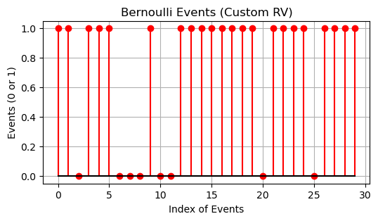
A Bernoulli random variable (RV) represents the simplest possible type of random variable, used for experiments with exactly two possible outcomes. These experiments are called Bernoulli trials, and the resulting random variable is referred to as a Bernoulli RV.
Characteristics#
Outcomes:
The two outcomes of a Bernoulli trial are typically assigned the values \( \{0, 1\} \), where:
\( 1 \): Represents success or the occurrence of a specific event.
\( 0 \): Represents failure or the non-occurrence of the event.
Probability Mass Function (PMF): If \( X \) is a Bernoulli RV, the PMF is given by:
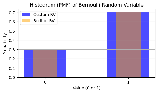
\[ p_X(0) = 1 - p, \quad p_X(1) = p \]where \( p \) (\( 0 \leq p \leq 1 \)) is the probability of success.
Probabilistic Representation:
The RV \( X \) takes the value:
\( 1 \) with probability \( p \).
\( 0 \) with probability \( 1 - p \).
Bernoulli random variables form the foundation for modeling binary outcomes in probabilistic experiments. Common applications include:
Coin tosses (e.g., heads or tails).
Binary decisions (e.g., yes or no).
Success-failure experiments in statistics.
Programming Resources
MATLAB: The Bernoulli distribution can be implemented using the function
binopdf.Python (SciPy): The Bernoulli distribution is available via
scipy.stats.bernoulli.
import numpy as np
import matplotlib.pyplot as plt
from scipy.stats import bernoulli

# Parameters
p = 0.7  # Probability of success
N = 10000  # Number of trials

# Simulate Bernoulli random variable using custom method
random_numbers = np.random.rand(N)  # Generate uniform random numbers
bernoulli_rv = (random_numbers <= p).astype(int)  # Bernoulli trials

# Simulate Bernoulli random variable using scipy.stats.bernoulli
bernoulli_builtin_rv = bernoulli.rvs(p, size=N)

# Empirical CDF calculation
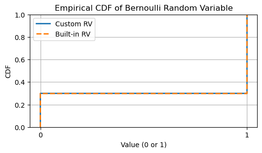
sorted_rv = np.sort(bernoulli_rv)
cdf_y = np.arange(1, N + 1) / N

# Visualization

# Bernoulli events plot (separate plots for empirical and built-in RVs)
plt.figure(figsize=(6, 3))
plt.stem(bernoulli_rv[:30], linefmt='r-', markerfmt='ro', basefmt="k", label='Custom RV')
plt.title('Bernoulli Events (Custom RV)')
plt.xlabel('Index of Events')
plt.ylabel('Events (0 or 1)')
plt.grid(True)

plt.figure(figsize=(6, 3))
plt.stem(bernoulli_builtin_rv[:30], linefmt='b-', markerfmt='bo', basefmt="k", label='Built-in RV')
plt.title('Bernoulli Events (Built-in RV)')
plt.xlabel('Index of Events')
plt.ylabel('Events (0 or 1)')
plt.grid(True)

# Histogram (PMF visualization)
plt.figure(figsize=(6, 3))
values, counts = np.unique(bernoulli_rv, return_counts=True)
probabilities = counts / N
plt.bar(values, probabilities, width=0.5, alpha=0.7, color='blue', label='Custom RV')
values_builtin, counts_builtin = np.unique(bernoulli_builtin_rv, return_counts=True)
probabilities_builtin = counts_builtin / N
plt.bar(values_builtin, probabilities_builtin, width=0.3, alpha=0.5, color='orange', label='Built-in RV')
plt.title('Histogram (PMF) of Bernoulli Random Variable')
plt.xlabel('Value (0 or 1)')
plt.ylabel('Probability')
plt.xticks([0, 1])
plt.legend()
plt.grid(axis='y')

# Empirical CDF plot
plt.figure(figsize=(6, 3))
plt.step(sorted_rv, cdf_y, where='post', linewidth=2, label='Custom RV')
sorted_builtin_rv = np.sort(bernoulli_builtin_rv)
cdf_builtin_y = np.arange(1, N + 1) / N
plt.step(sorted_builtin_rv, cdf_builtin_y, where='post', linewidth=2, linestyle='--', label='Built-in RV')
plt.title('Empirical CDF of Bernoulli Random Variable')
plt.xlabel('Value (0 or 1)')
plt.ylabel('CDF')
plt.ylim([0, 1])
plt.xticks([0, 1])
plt.legend()
plt.grid(True)

Gaussian Random Variable#
Importance of Gaussian Random Variables
Prevalence in Applications: The Gaussian random variable (RV) is the most widely used and significant RV in probability and statistics due to its universal applicability in modeling real-world phenomena.
Modeling Physical Phenomena: Many natural and engineered processes can be accurately modeled using Gaussian RVs. For example, thermal noise in electronic circuits and errors in measurements are often represented by Gaussian distributions.
Definition#
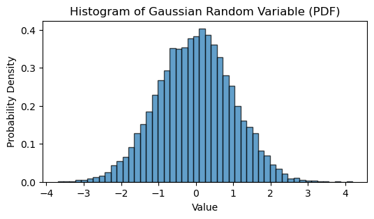
A Gaussian random variable is characterized by its probability density function (PDF), which has the general form:
This function describes the distribution of the variable \( X \) in terms of its central tendency and spread.
Key Parameters of the PDF#
Mean (\( m \)):
Represents the central location or average value of the Gaussian RV.
The distribution is symmetric around this point.
Standard Deviation (\( \sigma \)):
Measures the spread or dispersion of the distribution.
A larger \( \sigma \) results in a wider, flatter distribution, while a smaller \( \sigma \) results in a narrower, sharper peak.
Variance (\( \sigma^2 \)):
Defined as the square of the standard deviation, it quantifies the variability of the RV.
Notation
The Gaussian random variable \( X \) is denoted as:
which reads: \( X \) is normally distributed with mean \( m \) and variance \( \sigma^2 \).
The Gaussian RV is foundational in probability and statistics because:
It arises naturally in many systems due to the central limit theorem, where the sum of a large number of independent random variables tends to follow a normal distribution.
Its mathematical simplicity and well-defined properties make it a core tool in analysis and modeling.
CDF of A Gaussian RV#
The Cumulative Distribution Function (CDF) of a Gaussian random variable (RV) is a critical tool for determining probabilities associated with the RV. Specifically, the CDF is required to calculate the probability that the Gaussian RV \( X \) lies above, below, or within a specific interval.
The CDF of a Gaussian RV is defined as:
where:
\( m \): Mean of the Gaussian RV.
\( \sigma^2 \): Variance of the Gaussian RV.
Technical Challenges
No Closed-Form Solution: It is impossible to express this integral in a closed form using elementary functions.
Despite this limitation, the Gaussian CDF remains widely used due to its importance in probability and statistics.
Approaches to Compute the CDF
Tabulated Values:
The CDF of a Gaussian RV has been extensively tabulated.
These tables provide precomputed values for standard Gaussian RVs (e.g., \( m = 0, \sigma = 1 \)).
Reference materials, such as [B3, Appendix E], contain such tables for practical use.
Numerical Approximation:
Modern computational tools can approximate the Gaussian CDF to a desired level of accuracy.
These routines are efficient and eliminate the need for manual table lookup.
Despite the lack of a closed-form expression, the Gaussian CDF is indispensable in statistical modeling, hypothesis testing, and signal processing. Numerical methods and tables ensure its usability across various applications, making the Gaussian RV a cornerstone of probability theory.
Standard Forms for Gaussian CDF Evaluation#
When calculating the Cumulative Distribution Function (CDF) of a Gaussian random variable (RV), it must first be expressed in one of several commonly used standard forms.
These forms simplify computations and are widely used in mathematics and engineering.
Error Function (\( \text{erf}(x) \)):
Defined as twice the integral of a normalized Gaussian function from 0 to \( x \).
Expressed as:
\[ \text{erf}(x) = \frac{2}{\sqrt{\pi}} \int_{0}^{x} \exp(-t^2) \, dt, \quad x \geq 0, \, \text{erf}(x) \in [0,1]. \]The substitution \( t = \frac{x}{\sqrt{2}\sigma} \) relates it to Gaussian probabilities.
Complementary Error Function (\( \text{erfc}(x) \)):
Defined as:
\[ \text{erfc}(x) = 1 - \text{erf}(x) = \frac{2}{\sqrt{\pi}} \int_{x}^{\infty} \exp(-t^2) \, dt. \]Complements the error function to account for probabilities beyond \( x \).
\(\Phi\)-function:
Represents the CDF of a standard normal RV (mean \( 0 \), variance \( 1 \)):
\[ \Phi(x) = \frac{1}{\sqrt{2\pi}} \int_{-\infty}^{x} \exp\left(-\frac{t^2}{2}\right) \, dt. \]
\( Q \)-function:
Describes the tail probability beyond a threshold \( x \):
\[ Q(x) = \frac{1}{\sqrt{2\pi}} \int_{x}^{\infty} \exp\left(-\frac{t^2}{2}\right) \, dt. \]
import numpy as np
import matplotlib.pyplot as plt
from scipy.stats import norm
from scipy.special import erf

# Parameters
mu = 0  # Mean
sigma = 1  # Standard deviation
N = int(1e4)  # Number of samples

# Generate Gaussian random variables
gaussianRV_sim = mu + sigma * np.random.randn(N)

# Plotting Histogram for Gaussian RV
plt.figure(figsize=(6, 3))
plt.hist(gaussianRV_sim, bins=50, density=True, alpha=0.7, edgecolor='black')
plt.title('Histogram of Gaussian Random Variable (PDF)')
plt.xlabel('Value')
plt.ylabel('Probability Density')
plt.show()

# Find indices where RV > 3
indices_above_3 = np.where(gaussianRV_sim > 3)[0]
print(f"Indices where Gaussian RV > 3: {indices_above_3}")

# Gaussian random variables using scipy's built-in normal distribution
gaussianRV_builtin = norm.rvs(loc=mu, scale=sigma, size=N)

# Plotting built-in Gaussian RV histogram
plt.figure(figsize=(6, 3))
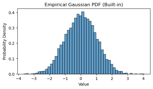
plt.hist(gaussianRV_builtin, bins=50, density=True, alpha=0.7, edgecolor='black')
plt.title('Empirical Gaussian PDF (Built-in)')
plt.xlabel('Value')
plt.ylabel('Probability Density')
plt.show()

# Empirical CDF for Gaussian RV
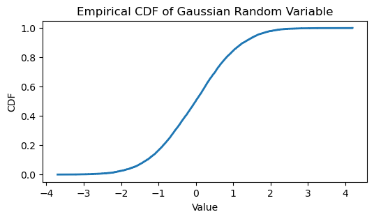
sorted_sim = np.sort(gaussianRV_sim)
ecdf_sim = np.arange(1, N + 1) / N

plt.figure(figsize=(6, 3))
plt.step(sorted_sim, ecdf_sim, where='post', linewidth=2)
plt.title('Empirical CDF of Gaussian Random Variable')
plt.xlabel('Value')
plt.ylabel('CDF')
plt.show()

# Theoretical PDF of Gaussian distribution
x_values = np.linspace(min(gaussianRV_sim), max(gaussianRV_sim), 1000)
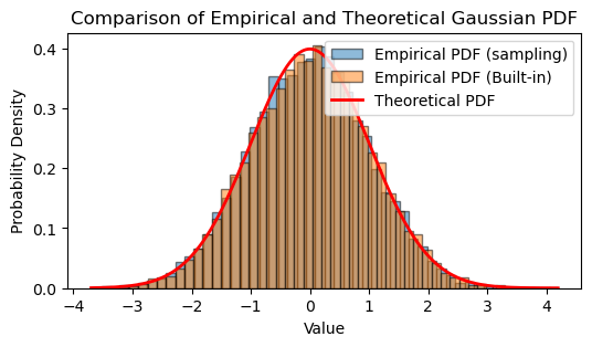
theoreticalPDF = (1 / (sigma * np.sqrt(2 * np.pi))) * np.exp(-0.5 * ((x_values - mu) / sigma)**2)

plt.figure(figsize=(6, 3))
plt.hist(gaussianRV_sim, bins=50, density=True, alpha=0.5, edgecolor='black', label='Empirical PDF (sampling)')
plt.hist(gaussianRV_builtin, bins=50, density=True, alpha=0.5, edgecolor='black', label='Empirical PDF (Built-in)')
plt.plot(x_values, theoreticalPDF, linewidth=2, color='r', label='Theoretical PDF')
plt.title('Comparison of Empirical and Theoretical Gaussian PDF')
plt.xlabel('Value')
plt.ylabel('Probability Density')
plt.legend()
plt.show()

# Theoretical CDF using the error function
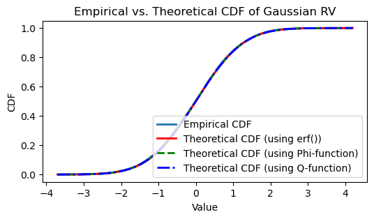
theoreticalCDF_erf = 0.5 * (1 + erf((x_values - mu) / (sigma * np.sqrt(2))))

# Theoretical CDF using Phi-function
def phi_function(x):
    return (1 / np.sqrt(2 * np.pi)) * np.exp(-0.5 * x**2)

theoreticalCDF_phi = np.cumsum(phi_function(x_values)) * (x_values[1] - x_values[0])

# Theoretical CDF using Q-function
def q_function(x):
    return 0.5 * (1 - erf(x / np.sqrt(2)))

theoreticalCDF_q = 1 - q_function((x_values - mu) / sigma)

# Plotting the CDFs
plt.figure(figsize=(6, 3))
plt.step(sorted_sim, ecdf_sim, where='post', linewidth=2, label='Empirical CDF')
plt.plot(x_values, theoreticalCDF_erf, 'r-', linewidth=2, label='Theoretical CDF (using erf())')
plt.plot(x_values, theoreticalCDF_phi, 'g--', linewidth=2, label='Theoretical CDF (using Phi-function)')
plt.plot(x_values, theoreticalCDF_q, 'b-.', linewidth=2, label='Theoretical CDF (using Q-function)')
plt.title('Empirical vs. Theoretical CDF of Gaussian RV')
plt.xlabel('Value')
plt.ylabel('CDF')
plt.legend()
plt.show()
Indices where Gaussian RV > 3: [ 244 828 1439 2282 5824 6021 7492 7641 7896 8976 8998 9452 9789]
Discussions on \( Q \)-Function#
Natural for Tail Probabilities:
The \( Q \)-function directly represents probabilities of the form \( \Pr(X > x) \), making it particularly useful for engineering applications.
Relation Between \( \Phi(x) \) and \( Q(x) \):
The \( Q \)-function is complementary to the \(\Phi\)-function:
\[ Q(x) = 1 - \Phi(x). \]
Expression of Gaussian CDF:
For a Gaussian RV \( X \sim \mathcal{N}(m, \sigma^2) \), the CDF can be expressed in terms of \( Q \):
\[ F_X(x) = \Pr(X \leq x) = 1 - Q\left( \frac{x - m}{\sigma} \right). \]
Advantages of Standard Forms#
Simplicity: Transforming a general Gaussian CDF to normalized forms like \( \Phi(x) \) or \( Q(x) \) simplifies numerical computations.
Common Usage: The \( Q \)-function is widely used in engineering and is supported by computational libraries and precomputed tables.
Practical Transformation: For a general Gaussian RV, the transformation \( t = \frac{x - m}{\sigma} \) allows easy evaluation of the CDF using normalized forms.
These standard forms ensure efficient and accurate evaluation of Gaussian probabilities in both theoretical and practical contexts.
Applications#
Mathematics vs. Engineering:
While the error function (\( \text{erf} \)) and complementary error function (\( \text{erfc} \)) are favored in mathematics, the \( Q \)-function is preferred in engineering due to its direct relevance to tail probabilities.
Efficient Computation:
Precomputed tables or numerical programs can efficiently evaluate the \( Q \)-function for practical applications.
