Correlation Receiver#
The optimal receiver for the AWGN channel follows the Maximum A Posteriori (MAP) decision rule, given by:
where the bias term is:
Here:
\( \vec{r} \) is the \( N \)-dimensional received vector.
\( \vec{s}_m \) is the \( m \)-th transmitted signal vector.
\( P_m \) is the prior probability of message \( m \).
\( \mathcal{E}_m = \|\vec{s}_m\|^2 \) is the signal energy.
\( N_0/2 \) is the noise power spectral density per dimension.
This rule selects the message \( m \) that maximizes the sum of a bias term (reflecting prior knowledge and signal energy) and the inner product \( \vec{r} \cdot \vec{s}_m \) (which measures alignment between the received and transmitted signals).
Implementing the MAP Decision Rule#
Extracting \( \vec{r} \) from the Received Waveform
A practical challenge arises because the receiver does not directly observe the vector \( \vec{r} \). Instead, it receives the continuous-time waveform:
where:
\( s_m(t) \) is the transmitted signal waveform.
\( n(t) \) is additive white Gaussian noise (AWGN).
To apply the MAP rule, the receiver must first extract the vector \( \vec{r} \) from \( r(t) \). This is achieved by projecting \( r(t) \) onto an orthonormal basis \( \{ \phi_j(t), 1 \leq j \leq N \} \), as established earlier using the Gram-Schmidt procedure.
The components of \( \vec{r} \) are computed as:
For each \( j \) (\( 1 \leq j \leq N \)), the receiver:
Multiplies the received signal \( r(t) \) by the basis function \( \phi_j(t) \).
Integrates over time, computing the projection of \( r(t) \) onto \( \phi_j(t) \).
Since the received signal is:
we obtain:
Breaking it down:
where:
\( s_{mj} = \int_{-\infty}^{\infty} s_m(t) \phi_j(t) \, dt \) is the \( j \)-th component of \( \vec{s}_m \).
\( n_j = \int_{-\infty}^{\infty} n(t) \phi_j(t) \, dt \) is the noise component, which is a Gaussian random variable with:
Zero mean.
Variance \( N_0/2 \).
This step transforms the continuous-time problem into an \( N \)-dimensional vector problem, making it compatible with the MAP detection rule.
Role of the Correlation Receiver#
The receiver’s integration process effectively correlates \( r(t) \) with each basis function \( \phi_j(t) \), extracting the necessary signal components. This explains why the optimal receiver in an AWGN channel is often referred to as a correlation receiver—it processes the received signal by computing inner products with known basis functions, enabling vector-based decision-making.
This correlation-based transformation is a fundamental concept in digital communication systems, linking waveform detection to vector-based statistical decision theory.
Operation of The Correlation Receiver#
Once the received vector is obtained as
the receiver executes the following sequence of operations:
Compute Inner Products
For each possible message \( m \) (from \( 1 \) to \( M \)), the receiver calculates the inner product between the received vector and each possible transmitted signal vector:
This dot product quantifies how well the received signal aligns with each potential transmitted signal. A higher inner product suggests a stronger match between \( \vec{r} \) and \( \vec{s}_m \).
Add Bias Terms
Each inner product is adjusted by adding a precomputed bias term:
This adjustment accounts for prior probabilities and signal energy differences. The final score for each possible transmitted message is:
Make a Decision
The receiver compares the scores across all \( M \) possible messages and selects the message index that maximizes the decision metric:
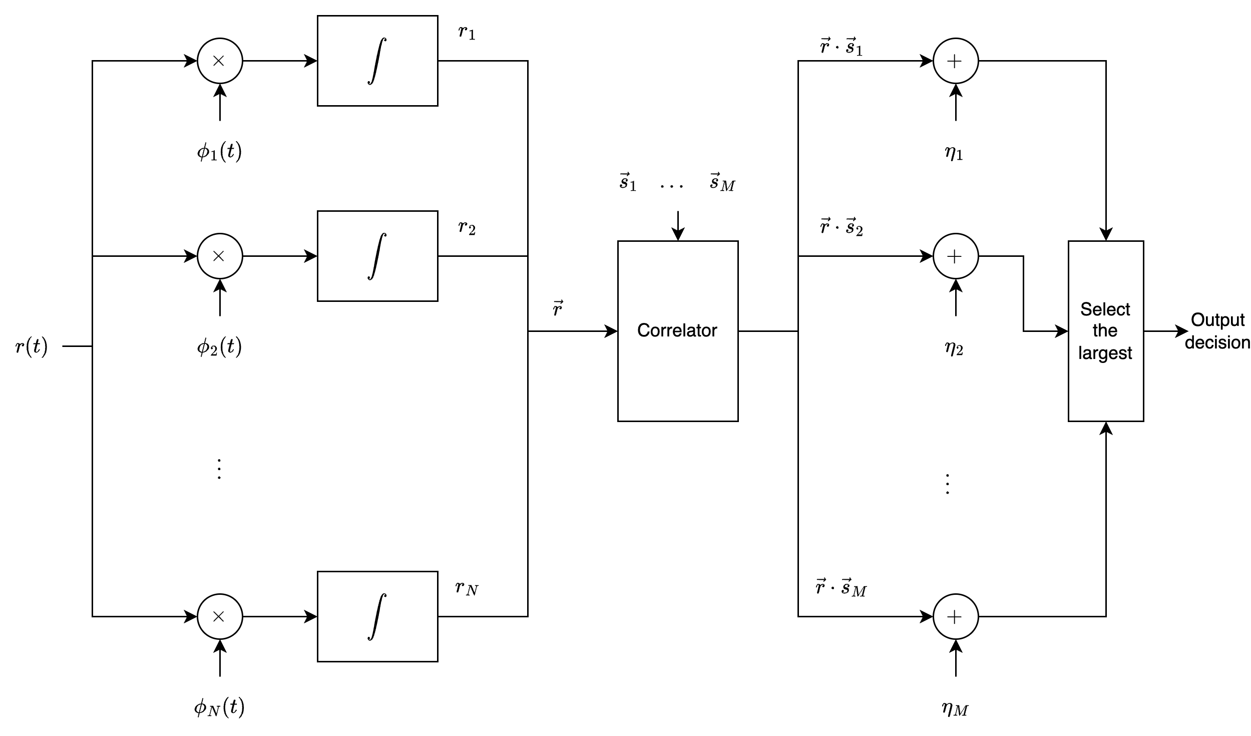 Illustration of a correlation receiver with \(N\) correlators.
Physical Meaning of The Correlation Receiver#
The first step involves correlating the received waveform \( r(t) \) with each basis function \( \phi_j(t) \), extracting the relevant signal components. The term “correlation receiver” reflects the use of inner products (or correlations) in this process.
Structural Overview of the Receiver
The receiver consists of \( N \) parallel correlators, each corresponding to a basis function \( \phi_j(t) \).
Each correlator computes \( r_j = \int_{-\infty}^{\infty} r(t) \phi_j(t) \, dt \), forming the vector \( \vec{r} \).
A computation stage then combines these outputs with the signal vectors \( \vec{s}_m \) and bias terms \( \eta_m \).
Finally, a maximum-selection operation determines the most likely transmitted message.
This correlation-based approach efficiently extracts the optimal decision statistics from the noisy received signal, making it fundamental in digital communication receivers.
Alternative Implementation#
A key practical advantage of the correlation receiver is that many components can be precomputed, significantly reducing the real-time computational load.
The bias terms
\[ \eta_m = \frac{N_0}{2} \ln P_m - \frac{1}{2} \mathcal{E}_m \]depend only on prior probabilities (\( P_m \)), noise power spectral density (\( N_0 \)), and signal energies (\( \mathcal{E}_m \)), all of which are system parameters independent of the received signal \( r(t) \).
The signal vectors
\[ \vec{s}_m = [s_{m1}, s_{m2}, \ldots, s_{mN}] \]where
\[ s_{mj} = \int_{-\infty}^{\infty} s_m(t) \phi_j(t) \, dt, \]are fixed for a given signal set and basis. These values can be precomputed and stored in memory, reducing real-time computation.
Dynamic Computation in the Receiver#
The only real-time computations required for each received \( r(t) \) are:
Generating \( \vec{r} \) via correlators, computing
\[ r_j = \int_{-\infty}^{\infty} r(t) \phi_j(t) \, dt \]for each basis function \( \phi_j(t) \).
Computing inner products
\[ \vec{r} \cdot \vec{s}_m = \sum_{j=1}^N r_j s_{mj} \]for each possible transmitted signal \( m \).
Alternative Implementation: Direct Time-Domain Correlation#
An alternative, yet equivalent, implementation bypasses the explicit computation of \( \vec{r} \cdot \vec{s}_m \) by directly correlating \( r(t) \) with each signal waveform \( s_m(t) \).
Starting from the inner product definition:
and substituting \( r_j \):
Using the signal expansion:
we obtain:
This follows from the linearity of integration and the orthonormality of the basis functions.
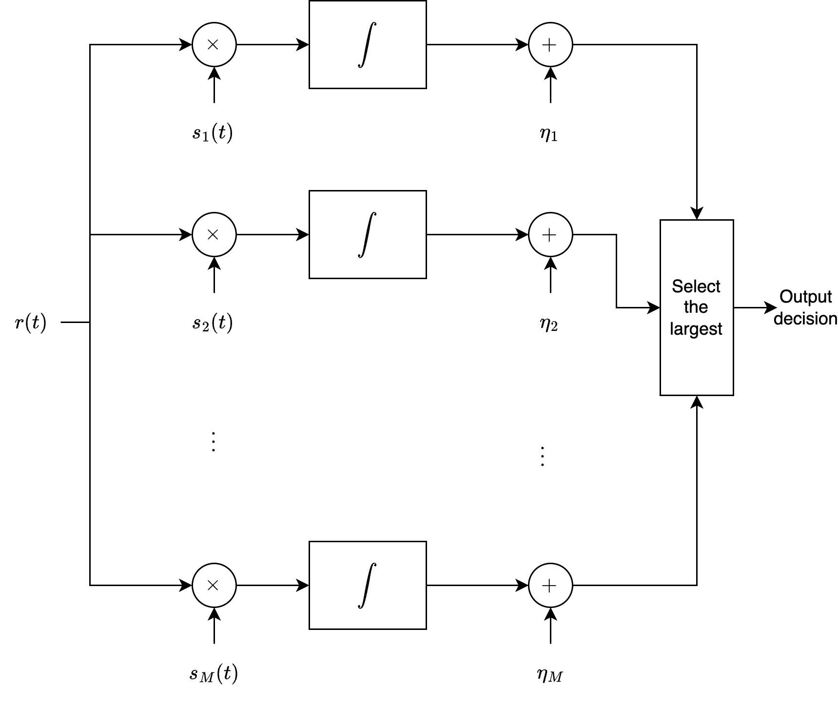 Illustration of a correlation receiver with \(M\) correlators in time domain.
MAP Decision Rule in Time Domain#
Instead of computing \( \vec{r} \) explicitly, the MAP rule can be rewritten as:
where
Comparison of Implementations
We can see that
Both approaches are mathematically equivalent but differ in implementation efficiency.
The vector-based approach is more structured and leverages precomputed signal vectors.
The direct time-domain correlation approach bypasses the explicit construction of \( \vec{r} \), potentially reducing computational complexity in some scenarios.
Second Version of the Correlation Receiver#
This alternative formulation leads to a second version of the correlation receiver, which restructures the detection process. Instead of using \( N \) correlators (one per basis function) followed by vector operations, this version employs \( M \) correlators—one for each possible transmitted signal waveform \( s_m(t) \).
Each correlator computes:
The resulting outputs are then adjusted by adding the corresponding bias terms \( \eta_m \), and the maximum value determines the detected message:
Intuition Behind the Second Version
This design is intuitive:
It directly matches the received signal against each possible transmitted waveform, without explicitly forming the received vector \( \vec{r} \).
It leverages the fact that each waveform \( s_m(t) \) is a linear combination of the basis functions weighted by the signal vector \( \vec{s}_m \).
Comparison with the First Version
Both implementations are mathematically equivalent, as they compute the same decision metric. However, the second version may be more efficient under certain conditions:
When \( M < N \) (fewer signals than dimensions):
The second version requires \( M \) correlators (one per signal) rather than \( N \) correlators (one per basis function).
This can reduce hardware complexity when the number of signals is smaller than the signal space dimension.
When the signal waveforms \( s_m(t) \) are readily available:
Some systems store entire waveforms rather than decomposing them into basis components.
The second version avoids precomputing and storing basis functions, simplifying implementation.