Comparison of Estimators#
MMSE estimator
MAP estimator
ML estimator
Summary of Previous Results#
Problem Statement
In this example, based on [B2, Ex 10.7], we want to find the estimate \(\hat{\boldsymbol{\mu}}\) of the unknown random mean \(\boldsymbol{\mu}\), using the set of observations \(\mathbf{y}_1, \ldots, \mathbf{y}_m\).
Assume further that the observations are statistically independent, normal random variables, each with unknown mean \(\boldsymbol{\mu}\) and known variance \(\sigma^2\).
The conditional pdf \(p(\vec{y}|\mu)\) is then
Next, assume that the a priori pdf \(p(\mu)\) is normal with mean \(m_1\) and variance \(\beta^2\), i.e.,
Note that the prior \( p(\mu) \) represents our knowledge about \(\mu\) before observing any data.
The MMSE, MAP, and ML estimates are, respectively:
Comparison of Estimators of Parameters
The first two estimates, \(\hat{\boldsymbol{\mu}}_{\text{MMSE}}\) and \(\hat{\boldsymbol{\mu}}_{\text{MAP}}\), are described as identical and biased.
The third estimate, \(\hat{\boldsymbol{\mu}}_{\text{ML}}\), is unbiased and efficient.
For large sample sizes \( m \) or large \( \beta^2 \), it is noted that \( \hat{\boldsymbol{\mu}}_{\text{MMSE}} (= \hat{\boldsymbol{\mu}}_{\text{MAP}}) \approx \bar{\mathbf{y}} = \hat{\boldsymbol{\mu}}_{\text{ML}} \) are approximately equal.
Large \( \beta^2 \) corresponds to an a priori probability density function (pdf) with a wide dispersion, meaning that little statistical information is gained from the prior knowledge.
In this case, the MMSE and MAP estimates reduce to the ML estimate, which does not require an a priori pdf.
import numpy as np
import matplotlib.pyplot as plt
import pandas as pd

# Set random seed for reproducibility (optional)
# np.random.seed(42)

# Parameters
m1 = 0.0        # Prior mean of mu
beta = 1.0      # Prior standard deviation of mu
sigma = 1.0     # Known standard deviation of observations
m = 10          # Number of observations per trial
k = 5          # Number of trials

# To store results
results = {
    'Trial': [],
    'True_mu': [],
    'Observations': [],
    'Sample_mean_y_bar': [],
    'MLE': [],
    'MAP': [],
    'MMSE': []
}

for trial in range(1, k + 1):
    # 1. Generate true mu based on prior
    true_mu = np.random.normal(m1, beta)

    # 2. Generate observations based on true mu
    observations = np.random.normal(true_mu, sigma, m)
    y_bar = np.mean(observations)

    # 3. Compute estimates
    # MLE: Sample mean
    mle = y_bar

    # MAP: (beta^2 * y_bar + sigma^2 * m1) / (beta^2 + sigma^2)
    map_estimate = (beta**2 * y_bar + sigma**2 * m1) / (beta**2 + sigma**2)

    # MMSE: Same as MAP in Gaussian case
    mmse = map_estimate

    # 4. Store the results
    results['Trial'].append(trial)
    results['True_mu'].append(true_mu)
    results['Observations'].append(observations)
    results['Sample_mean_y_bar'].append(y_bar)
    results['MLE'].append(mle)
    results['MAP'].append(map_estimate)
    results['MMSE'].append(mmse)

    # 5. Print the results for the current trial
    observations_str = np.array2string(observations, precision=4, separator=', ', suppress_small=True)
    print(f"Trial {trial}:")
    print(f"True μ: {true_mu:.4f}")
    print(f"Observations (vector y): {observations_str}")
    print(f"Statistic (sample mean ȳ): {y_bar:.4f}")
    print(f"MLE Estimate: {mle:.4f}")
    print(f"MAP Estimate: {map_estimate:.4f}")
    print(f"MMSE Estimate: {mmse:.4f}\n")

# Convert results to a DataFrame for better visualization
# Since 'Observations' is an array, we'll keep it as is or process separately if needed
df_results = pd.DataFrame({
    'Trial': results['Trial'],
    'True_mu': results['True_mu'],
    'Sample_mean_y_bar': results['Sample_mean_y_bar'],
    'MLE': results['MLE'],
    'MAP': results['MAP'],
    'MMSE': results['MMSE']
})

# Display the results table
print("Summary of Results:")
print(df_results.to_string(index=False))

# Visualization: Compare estimates with true mu across trials
plt.figure(figsize=(12, 6))
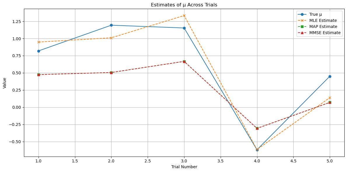
plt.plot(df_results['Trial'], df_results['True_mu'], marker='o', label='True μ')
plt.plot(df_results['Trial'], df_results['MLE'], marker='x', linestyle='--', label='MLE Estimate')
plt.plot(df_results['Trial'], df_results['MAP'], marker='s', linestyle='--', label='MAP Estimate')
plt.plot(df_results['Trial'], df_results['MMSE'], marker='^', linestyle='--', label='MMSE Estimate')
plt.title('Estimates of μ Across Trials')
plt.xlabel('Trial Number')
plt.ylabel('Value')
plt.legend()
plt.grid(True)
plt.tight_layout()
plt.show()

# Optional: Compute and display estimation errors
df_results['MLE_Error'] = df_results['MLE'] - df_results['True_mu']
df_results['MAP_Error'] = df_results['MAP'] - df_results['True_mu']
df_results['MMSE_Error'] = df_results['MMSE'] - df_results['True_mu']

print("\nEstimation Errors:")
print(df_results[['Trial', 'MLE_Error', 'MAP_Error', 'MMSE_Error']].to_string(index=False))

# Optional: Plot estimation errors
plt.figure(figsize=(12, 6))
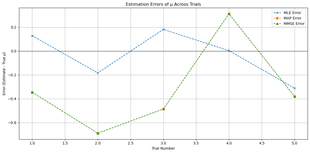
plt.plot(df_results['Trial'], df_results['MLE_Error'], marker='x', linestyle='--', label='MLE Error')
plt.plot(df_results['Trial'], df_results['MAP_Error'], marker='s', linestyle='--', label='MAP Error')
plt.plot(df_results['Trial'], df_results['MMSE_Error'], marker='^', linestyle='--', label='MMSE Error')
plt.axhline(0, color='black', linewidth=0.8)
plt.title('Estimation Errors of μ Across Trials')
plt.xlabel('Trial Number')
plt.ylabel('Error (Estimate - True μ)')
plt.legend()
plt.grid(True)
plt.tight_layout()
plt.show()
Trial 1:
True μ: 0.8193
Observations (vector y): [ 2.1743,  0.905 ,  1.6846,  0.0631,  1.1597,  1.6086,  2.9175, -0.4643,
 -0.7197,  0.1486]
Statistic (sample mean ȳ): 0.9477
MLE Estimate: 0.9477
MAP Estimate: 0.4739
MMSE Estimate: 0.4739

Trial 2:
True μ: 1.1935
Observations (vector y): [-0.379 ,  3.1874, -0.6197,  1.6783,  0.7355, -0.5886,  2.1176,  1.289 ,
  0.8837,  1.7972]
Statistic (sample mean ȳ): 1.0101
MLE Estimate: 1.0101
MAP Estimate: 0.5051
MMSE Estimate: 0.5051

Trial 3:
True μ: 1.1528
Observations (vector y): [ 2.6225,  0.9805, -0.1892,  2.4647,  0.8227,  1.5908,  0.3552,  2.4536,
  1.2346,  1.0021]
Statistic (sample mean ȳ): 1.3337
MLE Estimate: 1.3337
MAP Estimate: 0.6669
MMSE Estimate: 0.6669

Trial 4:
True μ: -0.6195
Observations (vector y): [-0.7227, -0.795 , -1.567 , -1.3811, -1.4331, -2.0088,  0.9924,  1.7117,
  1.1856, -2.1459]
Statistic (sample mean ȳ): -0.6164
MLE Estimate: -0.6164
MAP Estimate: -0.3082
MMSE Estimate: -0.3082

Trial 5:
True μ: 0.4501
Observations (vector y): [ 2.5458,  0.4679,  1.1959, -1.2552, -1.0884, -0.1493, -1.6052, -1.8537,
  2.4189,  0.7099]
Statistic (sample mean ȳ): 0.1387
MLE Estimate: 0.1387
MAP Estimate: 0.0693
MMSE Estimate: 0.0693

Summary of Results:
 Trial   True_mu  Sample_mean_y_bar       MLE       MAP      MMSE
     1  0.819300           0.947741  0.947741  0.473871  0.473871
     2  1.193471           1.010134  1.010134  0.505067  0.505067
     3  1.152803           1.333739  1.333739  0.666869  0.666869
     4 -0.619528          -0.616388 -0.616388 -0.308194 -0.308194
     5  0.450150           0.138650  0.138650  0.069325  0.069325
Estimation Errors:
 Trial  MLE_Error  MAP_Error  MMSE_Error
     1   0.128441  -0.345429   -0.345429
     2  -0.183338  -0.688404   -0.688404
     3   0.180936  -0.485934   -0.485934
     4   0.003140   0.311334    0.311334
     5  -0.311499  -0.380825   -0.380825
Example: Signal Reception in Noise#
In this example, based on [B2, Ex 10.20], we consider the reception of a signal embedded in noise, a common scenario in communications theory.
Problem Statement
We have \( L \) independent observations (or received-signal samples) \( \mathbf{y}_i \), which are expressed as the sum of a random signal \( \mathbf{s} \) and noise samples \( \mathbf{n}_i \):
Assumptions and PDFs
The random signal \( \mathbf{s} \) is uniformly distributed in the interval \( (0, a) \).
The pdf of the signal \( s \) is given by:
The random noise \( \mathbf{n}_i \) is Gaussian with zero mean and variance \( \sigma^2 \).
The pdf of the noise \( \mathbf{n}_i \) is:
Conditional Distribution of \( \mathbf{y}_i \) given \( s \)
For a constant \( s \), \( \mathbf{y}_i \) is Gaussian with mean \( s \) and variance \( \sigma^2 \).
Thus, the pdf \( p(\vec{y} | s) \) can be written as:
Task
We want to estimate the random \(\mathbf{s}\).
import numpy as np
import matplotlib.pyplot as plt

# Parameters
a = 1          # Upper bound for the true signal
sigma = 1    # Standard deviation of the noise
L = 10         # Number of observations per trial
k = 5          # Number of trials

# To store signals and observations for analysis
signals = []
observations = []

for trial in range(1, k + 1):
    # Generate a random true signal within (0, a)
    signal = np.random.uniform(0, a)

    # Generate Gaussian noise
    noise = np.random.normal(0, sigma, L)

    # Generate observations by adding noise to the signal
    y = signal + noise

    # Store the results
    signals.append(signal)
    observations.append(y)

    # Display the results for the current trial
    print(f"Trial {trial}:")
    print(f"True Signal (fixed parameter s): {signal:.4f}")
    print(f"Observations (vector y): {y}\n")
Trial 1:
True Signal (fixed parameter s): 0.4516
Observations (vector y): [ 1.32064602 -0.5077289  -0.66214343  1.44271647 -0.82477021  1.81397064
 -0.80037337 -0.19763709  0.37709459  0.27959563]

Trial 2:
True Signal (fixed parameter s): 0.2683
Observations (vector y): [-0.52152635  0.38722607  0.35052791  1.02839825  1.951469   -0.62050193
  0.63186598 -0.77860689  1.50367162 -0.24161981]

Trial 3:
True Signal (fixed parameter s): 0.1999
Observations (vector y): [ 1.43114502 -1.42366952 -0.05386208  0.39046     0.04691115  1.44249959
 -1.57316783  0.05206321  0.56235636  0.17916296]

Trial 4:
True Signal (fixed parameter s): 0.3236
Observations (vector y): [-1.7656375   1.89771449 -0.05695857  0.94111807  2.5332734  -0.54548923
 -0.80319628 -0.61812149  0.46580735 -0.09023442]

Trial 5:
True Signal (fixed parameter s): 0.0654
Observations (vector y): [ 0.00732296  0.30873143 -1.37173128  1.80500289 -0.22437932 -0.70756438
  0.8684864   1.24873887  0.26297671  1.87421202]
Method 1: Maximum Likelihood Estimate#
Recall that the Maximum Likelihood Estimator seeks the value of \( s \) that maximizes the likelihood of the observed data \( \vec{y} = (y_1, y_2, \dots, y_L) \).
Mathematically, the ML estimator is given by:
Unlike MAP estimation, ML does not consider the prior distribution \( p(s) \).
Finding \( \hat{s}_{\text{ML}} \)#
We need to maximize the likelihood \( p(\vec{y} | s) \) with respect to \( s \).
Maximizing the likelihood is equivalent to maximizing the log-likelihood since the logarithm is a monotonically increasing function.
The log-likelihood \( \mathcal{L}(s) \) is:
To maximize \( \mathcal{L}(s) \), we can equivalently minimize the negative log-likelihood:
This is a quadratic function in \( s \), which is minimized when its derivative with respect to \( s \) is zero.
Compute the derivative of the sum of squared errors with respect to \( s \):
Set the derivative to zero for minimization:
Simplifying:
where \( \bar{y} \) is the sample mean of the observations.
The Maximum Likelihood Estimator for \( s \) is the sample mean of the observations:
In general
where \( \bar{\mathbf{y}} \) is the sample mean.
Note that, unless explicitly stated, ML estimation typically assumes an unconstrained parameter space.
Method 2: Maximum A Posteriori Estimate (MAP)#
The MAP estimator seeks the value of \( s \) that maximizes the posterior distribution \( p(s | \vec{y}) \), where \( \vec{y} = (y_1, y_2, \dots, y_L) \) represents all observations.
Mathematically, the MAP estimator is given by:
By Bayes’ theorem:
Since \( p(\vec{y}) \) is constant with respect to \( s \), maximizing \( p(s | \vec{y}) \) is equivalent to maximizing the product of the likelihood \( p(\vec{y} | s) \) and the prior \( p(s) \):
Combining the likelihood and the prior, the MAP estimator maximizes:
Substituting the expressions:
Since \( \left( \frac{1}{\sqrt{2\pi \sigma^2}} \right)^L \) and \( \frac{1}{a} \) are constants (when \( 0 < s < a \)), maximizing the above expression reduces to minimizing the exponent term within the allowed range of \( s \):
Solving the differential equation#
The expression to minimize is a quadratic function in \( s \):
Taking the derivative with respect to \( s \) and setting it to zero to find the minimum:
Solving for \( s \):
where \( \bar{y} \) is the sample mean of the observations.
The MAP estimator must respect the prior constraints \( 0 < s < a \). Therefore, the estimator is:
This can be compactly written using the clipping (or saturation) function:
Putting it all together, the MAP estimator for \( s \) is:
Method 3: Minimum Mean Squared Error (MMSE) Estimate#
Problem Formulation#
The MMSE Estimator seeks to minimize the mean squared error between the estimated signal \( \hat{s} \) and the true signal \( s \). Mathematically, it is defined as:
Using Bayesian estimation, this expectation can be expressed as:
Substituting the expressions for \( p(\vec{y}|s) \) and \( p(s) \) into the MMSE formula:
Given the support of \( p(s) \) is \( (0, a) \), the integrals simplify to:
Since \( \frac{1}{a} \) is a constant, it cancels out in the numerator and denominator:
Notice that:
where \( \bar{y} = \frac{1}{L} \sum_{i=1}^{L} y_i \) is the sample mean.
Thus, the joint likelihood becomes:
The term \( \sum_{i=1}^{L} (y_i - \bar{y})^2 \) is independent of \( s \), so it acts as a constant in both the numerator and denominator and cancels out. Therefore:
Derivation of the MMSE Estimate#
To evaluate the integrals, perform a change of variables to standardize the Gaussian exponent.
Let:
Thus:
Constraints from the prior probability \(p(s)\):
When \( s = 0 \):
\[ z_1 = \frac{ 0 - \bar{y} }{ \tau } = -\frac{ \bar{y} \sqrt{L} }{ \sigma } \]When \( s = a \):
\[ z_2 = \frac{ a - \bar{y} }{ \tau } = \frac{ (a - \bar{y}) \sqrt{L} }{ \sigma } \]
Substituting into the integrals:
Simplifying, the \( \tau \) terms cancel out:
Split the numerator:
For the first integral
where \( \Phi(z) \) is the standard normal cumulative distribution function (CDF), i.e., \(\Phi(z) = 1- Q(z)\).
For the second integral
Thus, the numerator becomes:
And the denominator is:
Therefore, the MMSE estimator is:
Recall that:
Substituting these back:
Simplifying:
Note: \( \Phi(-x) = 1 - \Phi(x) \), so:
Thus, the denominator can be rewritten as:
Therefore, the MMSE estimator simplifies to:
Alternatively, using the error function \( \text{erf}(x) \), which is related to the standard normal CDF \( \Phi(x) \) by:
We can express the MMSE estimator as:
Simplifying the denominator:
Thus, the MMSE estimator becomes:
This expression neatly encapsulates the MMSE estimator in terms of the sample mean \( \bar{y} \), the error function, and the system parameters \( a \), \( \sigma \), and \( L \).
Summary: Expressions for the MMSE Estimator
To present the MMSE estimator in a compact and interpretable form, we can express it as:
Alternatively, using the error function \( \text{erf}(x) \):
where
\( \bar{y} = \frac{1}{L} \sum_{i=1}^{L} y_i \) is the sample mean.
\( \Phi(x) \) is the standard normal CDF.
\( \text{erf}(x) \) is the error function, related to the standard normal CDF by:
\[ \Phi(x) = \frac{1}{2} \left[ 1 + \text{erf}\left( \frac{x}{\sqrt{2}} \right) \right] \]
Example Calculation#
Given:
\( L = 10 \) observations:
\[ \vec{y} = [2.0, 2.2, 1.8, 2.1, 2.3, 2.0, 2.1, 2.2, 1.9, 2.0] \]\( a = 3 \)
\( \sigma = 0.5 \)
Calculate the Sample Mean:
Compute the MMSE Estimator:
Substitute the values into the MMSE estimator formula:
Calculating each component:
Exponentials
CDFs
Thus:
Substituting Back
Thus, we have
Since the sample mean \( \bar{y} = 2.06 \) lies well within the interval \( (0, 3) \), the MMSE estimator closely aligns (not identical, because this is an approximation) with the sample mean, as expected.
Biasness of MMSE#
Bias: The final expression shows that the MMSE estimate \( \hat{s}_{MS} \) is biased. This contrasts with the ML and MAP estimates, which are unbiased.
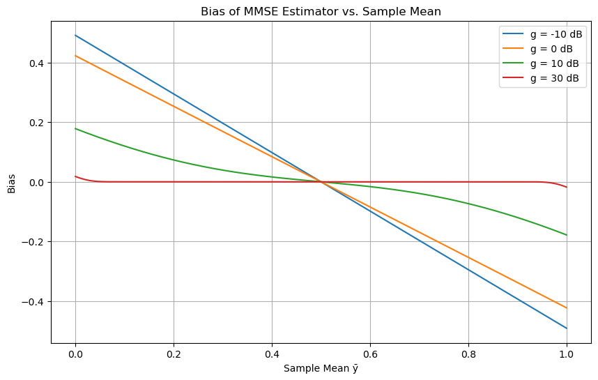
The bias term (involving \( \bar{y} \)) can be numerically evaluated to show how its bias is affected by a parameter defined in decibels (dB).
The quality of the estimate depends on the parameter \( L / (2\sigma^2) \), which is expressed in decibels as:
The MMSE estimator expressed as a function of \( g = \frac{L}{2\sigma^2} \) (linear) as
import numpy as np
import matplotlib.pyplot as plt
from scipy.special import erf

# Define the MMSE estimator function
def mmse_estimator(y_bar, g, a=1):
    numerator = np.exp(-g * y_bar**2) - np.exp(-g * (a - y_bar)**2)
    denominator = erf((a - y_bar) * np.sqrt(g)) + erf(y_bar * np.sqrt(g))
    # To handle division by zero, we add a small epsilon to the denominator
    epsilon = 1e-12
    denominator = np.where(denominator == 0, epsilon, denominator)
    estimator = y_bar + (1 / np.sqrt(np.pi * g)) * (numerator / denominator)
    return estimator

# Parameters
a = 1
y_bar = np.linspace(0, a, 1000)
g_dB_values = [-10, 0, 10, 30]
g_values = 10 ** (np.array(g_dB_values) / 10)

# Plotting
plt.figure(figsize=(10, 6))
for g_dB, g in zip(g_dB_values, g_values):
    estimator = mmse_estimator(y_bar, g, a)
    bias = estimator - y_bar
    plt.plot(y_bar, bias, label=f'g = {g_dB} dB')

plt.title('Bias of MMSE Estimator vs. Sample Mean')
plt.xlabel('Sample Mean ȳ')
plt.ylabel('Bias')
plt.legend()
plt.grid(True)
plt.show()
Schonhoff’s Method#
import numpy as np
import matplotlib.pyplot as plt
from scipy.stats import norm

def bias(gdb):
    """
    Calculate the bias of the MMSE Estimate for a given gdb.

    Parameters:
        gdb (float): g in decibels, defined as 10 * log10(L / (2 * sigma^2))

    Returns:
        b (numpy.ndarray): Bias of the MMSE estimate for y ranging from 0 to 1 in steps of 0.1
    """
    # Convert gdb from decibels to linear scale
    g = 10**(0.1 * gdb)

    # Calculate coefficients
    coef = 1 / np.sqrt(np.pi * g)
    sig = 1 / np.sqrt(2 * g)

    # Initialize bias array
    b = np.zeros(11)

    # Calculate bias for y values from 0 to 1 in steps of 0.1
    for k in range(1, 12):
        y = (k - 1) * 0.1
        t1 = np.exp(-y**2 * g)
        t2 = np.exp(-(y - 1)**2 * g)

        if np.isclose(t1, t2):
            b[k-1] = 0
        else:
            td1 = norm.cdf(y, loc=0, scale=sig)
            td2 = norm.cdf(y, loc=1, scale=sig)
            denominator = 2 * (td1 - td2)

            # To avoid division by zero, check if denominator is not zero
            if not np.isclose(denominator, 0):
                b[k-1] = coef * (t1 - t2) / denominator
            else:
                b[k-1] = 0  # Assign zero or handle as needed

    return b

def plot_bias(gdb_values, y_range=(0, 1), step=0.1):
    """
    Plot the bias of the MMSE Estimate for multiple gdb values.

    Parameters:
        gdb_values (list or array-like): List of gdb values in decibels to plot
        y_range (tuple): The range of y values (start, end)
        step (float): Step size for y values
    """
    # Create y-axis values based on the specified range and step
    y_values = np.arange(y_range[0], y_range[1] + step, step)

    plt.figure(figsize=(10, 7))

    for gdb in gdb_values:
        bias_values = bias(gdb)
        plt.plot(y_values, bias_values, linestyle='-', label=f'gdb = {gdb} dB')

    plt.grid(True, which='both', linestyle='--', linewidth=0.5)
    plt.xlabel('Sample Mean ȳ', fontsize=12)
    plt.ylabel('Bias', fontsize=12)
    plt.title('Bias of MMSE Estimate for Various gdb Values', fontsize=14)
    plt.legend(title='gdb Values', fontsize=10)
    plt.tight_layout()
    plt.show()

# Example usage
if __name__ == "__main__":
    # Define multiple gdb values
    gdb_values = [-10, 0, 10, 30]  # You can add more values as needed

    # Plot bias for the specified gdb values
    plot_bias(gdb_values)
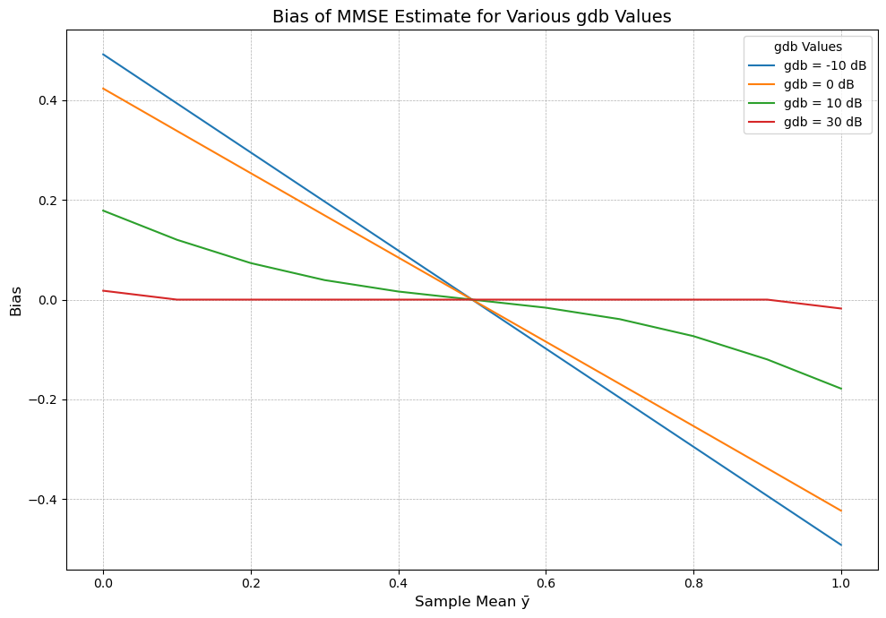
The bias decreases as \( g_{dB} \) increases, and as \( g_{dB} \) becomes large, the bias term approaches zero, meaning the MMSE estimate becomes closer to unbiased.
We can say that the larger the signal-to-noise ratio (expressed by \( g_{dB} \)), the smaller the bias in the MMSE estimate.
Discussion#
Data Integration: The MMSE estimator \( \hat{s}_{\text{MMSE}} \) integrates both the observed data (through the sample mean \( \bar{y} \)) and the prior information about \( s \) (uniformly distributed over \( (0, a) \)). This ensures that the estimator not only fits the data but also adheres to the known constraints on \( s \).
Bias-Variance Trade-off: Unlike the Maximum Likelihood estimator, which solely relies on data and can be biased when data suggests estimates outside \( (0, a) \), the MMSE estimator incorporates prior knowledge to potentially introduce bias that reduces the overall mean squared error.
Behavior Near Boundaries:
Central Estimates (\( \bar{y} \) well within \( (0, a) \)): The MMSE estimator closely aligns with the sample mean, similar to the ML estimator.
Boundary Estimates (\( \bar{y} \) near 0 or \( a \)): The estimator adjusts the estimate to respect the prior constraints, preventing it from exceeding the bounds. This results in a smoother transition compared to the ML estimator, which might abruptly clip estimates.
Simulation of 3 Methods#
import numpy as np
import matplotlib.pyplot as plt
from scipy.stats import norm
from scipy.integrate import quad
from scipy.special import erf

# Simulation Parameters
L = 10              # Number of observations
a = 3.0             # Upper bound for s
sigma = 2         # Noise standard deviation
num_trials = 1000  # Number of simulation trials

# Function to compute MMSE estimator via numerical integration
def mmse_estimator_numerical(y_bar, L, sigma, a):
    # Define the integrand for the numerator: s * exp(- (L/(2*sigma^2)) * (s - y_bar)^2)
    def numerator_integrand(s):
        return s * np.exp(- (L / (2 * sigma**2)) * (s - y_bar)**2)

    # Define the integrand for the denominator: exp(- (L/(2*sigma^2)) * (s - y_bar)^2)
    def denominator_integrand(s):
        return np.exp(- (L / (2 * sigma**2)) * (s - y_bar)**2)

    # Compute the integrals numerically
    numerator, _ = quad(numerator_integrand, 0, a, limit=100)
    denominator, _ = quad(denominator_integrand, 0, a, limit=100)

    # Avoid division by zero
    if denominator == 0:
        return 0
    else:
        return numerator / denominator

# Function to compute MMSE estimator via closed-form expression
def mmse_estimator_closed_form(y_bar, L, sigma, a):
    # Compute the exponent terms
    exponent1 = - (y_bar ** 2) * L / (2 * sigma ** 2)
    exponent2 = - ((a - y_bar) ** 2) * L / (2 * sigma ** 2)

    # Compute the numerator and denominator
    numerator = np.exp(exponent1) - np.exp(exponent2)

    # Compute the error functions
    erf1 = erf((a - y_bar) * np.sqrt(L) / (sigma * np.sqrt(2)))
    erf2 = erf(y_bar * np.sqrt(L) / (sigma * np.sqrt(2)))

    # Compute the denominator of the fraction inside the formula
    denominator = 0.5 * (erf1 + erf2)

    # Avoid division by zero
    if denominator == 0:
        adjustment = 0
    else:
        adjustment = (sigma / np.sqrt(2 * np.pi * L)) * (numerator / denominator)

    # Compute the closed-form MMSE estimator
    s_mmse_closed = y_bar + adjustment
    return s_mmse_closed

# Function to compute MAP estimator via theory
def map_estimator_closed_form(y_bar, a):
    return min(a, max(0, y_bar))

# Function to compute MAP estimator via numerical root-finding (generalized approach)
def map_estimator_numerical(y_bar, L, sigma, a):
    # Define the derivative of log p(s | y) with respect to s
    def derivative_log_posterior(s):
        # For uniform prior, p(s) is constant within [0, a]
        # So derivative is same as derivative of log p(y | s)
        # p(y | s) ~ exp(- (sum (y_i - s)^2)/(2 sigma^2))
        # derivative: d/ds log p(y | s) = sum (y_i - s) / sigma^2 = L (y_bar - s) / sigma^2
        return L * (y_bar - s) / (sigma ** 2)

    # Attempt to find the root within [0, a]
    # Given the derivative is linear in s, the root is at s = y_bar
    # Clamp the root to [0, a]
    s_root = y_bar
    s_root_clamped = min(a, max(0, s_root))
    return s_root_clamped

# Initialize arrays to store results
ml_estimates = np.zeros(num_trials)
map_estimates_closed_form = np.zeros(num_trials)
map_estimates_numerical = np.zeros(num_trials)
mmse_estimates_numerical = np.zeros(num_trials)
mmse_estimates_closed = np.zeros(num_trials)
true_signals = np.zeros(num_trials)

# Simulation Loop
for trial in range(num_trials):
    # Randomly choose a true signal s within (0, a)
    s = np.random.uniform(0, a)
    true_signals[trial] = s

    # Generate L observations with Gaussian noise
    y = s + np.random.normal(0, sigma, L)
    y_bar = np.mean(y)

    # ML Estimator
    s_ml = y_bar
    ml_estimates[trial] = s_ml

    # MAP Estimator via Closed-Form
    s_map_proj = map_estimator_closed_form(y_bar, a)
    map_estimates_closed_form[trial] = s_map_proj

    # MAP Estimator via Numerical Root-Finding
    s_map_num = map_estimator_numerical(y_bar, L, sigma, a)
    map_estimates_numerical[trial] = s_map_num

    # MMSE Estimator via Numerical Integration
    s_mmse_num = mmse_estimator_numerical(y_bar, L, sigma, a)
    mmse_estimates_numerical[trial] = s_mmse_num

    # MMSE Estimator via Closed-Form Expression
    s_mmse_closed = mmse_estimator_closed_form(y_bar, L, sigma, a)
    mmse_estimates_closed[trial] = s_mmse_closed

# Compute Squared Errors
ml_errors = (true_signals - ml_estimates) ** 2
map_errors_proj = (true_signals - map_estimates_closed_form) ** 2
map_errors_num = (true_signals - map_estimates_numerical) ** 2
mmse_errors_num = (true_signals - mmse_estimates_numerical) ** 2
mmse_errors_closed_form = (true_signals - mmse_estimates_closed) ** 2

# Compute Mean Squared Errors
mse_ml = np.mean(ml_errors)
mse_map_proj = np.mean(map_errors_proj)
mse_map_num = np.mean(map_errors_num)
mse_mmse_num = np.mean(mmse_errors_num)
mse_mmse_closed = np.mean(mmse_errors_closed_form)

print(f"Mean Squared Error (ML Estimator): {mse_ml:.5f}")
print(f"Mean Squared Error (MAP Estimator - Closed-Form): {mse_map_proj:.5f}")
print(f"Mean Squared Error (MAP Estimator - Numerical): {mse_map_num:.5f}")
print(f"Mean Squared Error (MMSE Estimator - Closed-Form): {mse_mmse_closed:.5f}")
print(f"Mean Squared Error (MMSE Estimator - Numerical): {mse_mmse_num:.5f}")
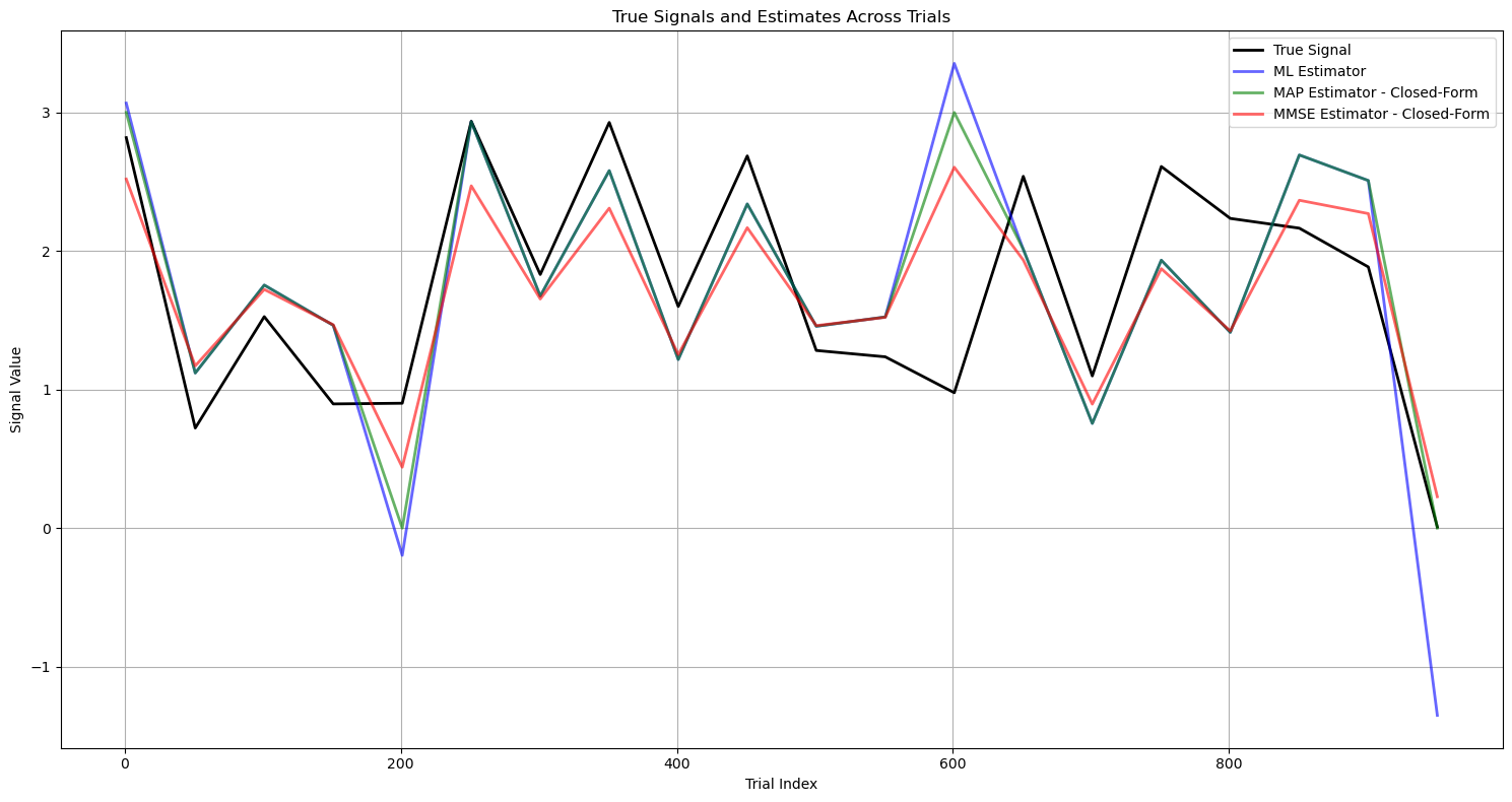
Mean Squared Error (ML Estimator): 0.41932
Mean Squared Error (MAP Estimator - Closed-Form): 0.32206
Mean Squared Error (MAP Estimator - Numerical): 0.32206
Mean Squared Error (MMSE Estimator - Closed-Form): 0.26368
Mean Squared Error (MMSE Estimator - Numerical): 0.26368
# Additional Plot: True Signals vs Selected Estimators with Trial Index on X-axis
# To visualize how estimates evolve over trials, we can plot the estimators against trial index.

# To make the plot readable, especially with huge trials, we'll plot a subset, e.g., every k-th trial.
subset_indices = np.arange(0, num_trials, 50)
subset_trials = subset_indices + 1  # Trial indices starting from 1

plt.figure(figsize=(15, 8))
plt.plot(subset_trials, true_signals[subset_indices],
         label='True Signal', color='black', linewidth=2)
plt.plot(subset_trials, ml_estimates[subset_indices],
         label='ML Estimator', color='blue', alpha=0.6, linewidth=2)
plt.plot(subset_trials, map_estimates_closed_form[subset_indices],
         label='MAP Estimator - Closed-Form', color='green', alpha=0.6, linewidth=2)
plt.plot(subset_trials, mmse_estimates_closed[subset_indices],
         label='MMSE Estimator - Closed-Form', color='red', alpha=0.6, linewidth=2)
plt.title('True Signals and Estimates Across Trials')
plt.xlabel('Trial Index')
plt.ylabel('Signal Value')
plt.legend()
plt.grid(True)
plt.tight_layout()
plt.show()
# Plotting Histograms of Squared Errors and True Signal vs Estimates in pairs

# Pair 1: ML Estimator
plt.figure(figsize=(12, 4))

plt.subplot(1, 2, 1)
plt.hist(ml_errors, bins=50, alpha=0.7, label='ML Estimator', color='blue', density=True)
plt.title('Histogram of Squared Errors (ML)')
plt.xlabel('Squared Error')
plt.ylabel('Density')
plt.legend()

plt.subplot(1, 2, 2)
plt.scatter(true_signals, ml_estimates, alpha=0.3, label='ML Estimator', color='blue', s=10)
plt.plot([0, a], [0, a], 'k--', label='Ideal')
plt.title('True Signal vs ML Estimates')
plt.xlabel('True Signal (s)')
plt.ylabel('Estimated Signal')
plt.legend()

plt.tight_layout()
plt.show()

# Pair 2: MAP Estimator - Closed-Form
plt.figure(figsize=(12, 4))

plt.subplot(1, 2, 1)
plt.hist(map_errors_proj, bins=50, alpha=0.7, label='MAP Estimator - Closed-Form', color='green', density=True)
plt.title('Histogram of Squared Errors (MAP - Closed-Form)')
plt.xlabel('Squared Error')
plt.ylabel('Density')
plt.legend()

plt.subplot(1, 2, 2)
plt.scatter(true_signals, map_estimates_closed_form, alpha=0.3, label='MAP Estimator - Closed-Form', color='green', s=10)
plt.plot([0, a], [0, a], 'k--', label='Ideal')
plt.title('True Signal vs MAP Estimates (Closed-Form)')
plt.xlabel('True Signal (s)')
plt.ylabel('Estimated Signal')
plt.legend()

plt.tight_layout()
plt.show()

# Pair 3: MMSE Estimator - Closed-Form
plt.figure(figsize=(12, 4))

plt.subplot(1, 2, 1)
plt.hist(mmse_errors_closed_form, bins=50, alpha=0.7, label='MMSE Estimator - Closed-Form', color='red', density=True)
plt.title('Histogram of Squared Errors (MMSE - Closed-Form)')
plt.xlabel('Squared Error')
plt.ylabel('Density')
plt.legend()

plt.subplot(1, 2, 2)
plt.scatter(true_signals, mmse_estimates_closed, alpha=0.3, label='MMSE Estimator - Closed-Form', color='red', s=10)
plt.plot([0, a], [0, a], 'k--', label='Ideal')
plt.title('True Signal vs MMSE Estimates (Closed-Form)')
plt.xlabel('True Signal (s)')
plt.ylabel('Estimated Signal')
plt.legend()

plt.tight_layout()
plt.show()


# To store y_bar for selected trials
selected_trials = [0, np.random.randint(0, num_trials)]  # First, random
selected_y_bars = []
selected_s_true = []

# Simulation Loop
for trial in range(num_trials):
    # Randomly choose a true signal s within (0, a)
    s = np.random.uniform(0, a)
    true_signals[trial] = s

    # Generate L observations with Gaussian noise
    y = s + np.random.normal(0, sigma, L)
    y_bar = np.mean(y)

    # ML Estimator
    s_ml = y_bar
    ml_estimates[trial] = s_ml

    # MAP Estimator via Closed-Form
    s_map_proj = map_estimator_closed_form(y_bar, a)
    map_estimates_closed_form[trial] = s_map_proj

    # MAP Estimator via Numerical Root-Finding
    s_map_num = map_estimator_numerical(y_bar, L, sigma, a)
    map_estimates_numerical[trial] = s_map_num

    # MMSE Estimator via Numerical Integration
    s_mmse_num = mmse_estimator_numerical(y_bar, L, sigma, a)
    mmse_estimates_numerical[trial] = s_mmse_num

    # MMSE Estimator via Closed-Form Expression
    s_mmse_closed = mmse_estimator_closed_form(y_bar, L, sigma, a)
    mmse_estimates_closed[trial] = s_mmse_closed

    # Store data for selected trials
    if trial in selected_trials:
        selected_y_bars.append(y_bar)
        selected_s_true.append(s)


# To make the plot readable, especially with huge trials, we'll plot a subset, e.g., every k-th trial.
subset_indices = np.arange(0, num_trials, 10)
subset_trials = subset_indices + 1  # Trial indices starting from 1


# Plotting PDFs for Selected Trials
for idx, trial in enumerate(selected_trials):
    s_true = selected_s_true[idx]
    y_bar = selected_y_bars[idx]

    # Define s range for plotting
    s_values = np.linspace(0, a, 500)

    # Prior p(s): Uniform distribution
    p_s = np.ones_like(s_values) / a  # Uniform on [0,a]

    # Likelihood p(y | s): Gaussian centered at y_bar with variance sigma^2 / L
    # Since y_bar is the sample mean of L observations, the likelihood of y_bar given s is N(s, sigma^2 / L)
    p_y_given_s = norm.pdf(y_bar, loc=s_values, scale=sigma / np.sqrt(L))

    # Posterior p(s | y): p(y | s) * p(s) normalized
    p_s_given_y = p_y_given_s * p_s
    p_s_given_y /= np.trapz(p_s_given_y, s_values)  # Normalize

    # Estimators
    s_ml = ml_estimates[trial]
    s_map = map_estimates_closed_form[trial]
    s_mmse = mmse_estimates_closed[trial]
# Plotting
plt.figure(figsize=(10, 6))
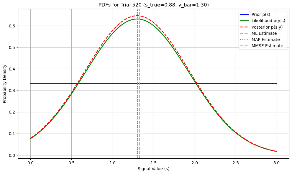
plt.plot(s_values, p_s, label='Prior p(s)', color='blue', linewidth=2)
plt.plot(s_values, p_y_given_s, label='Likelihood p(y|s)', color='green', linewidth=2, linestyle='-')
plt.plot(s_values, p_s_given_y, label='Posterior p(s|y)', color='red', linewidth=2, linestyle='--')

# Mark estimators on the posterior
plt.axvline(s_ml, color='cyan', linestyle='--', linewidth=2, label='ML Estimate')
plt.axvline(s_map, color='magenta', linestyle=':', linewidth=2, label='MAP Estimate')
plt.axvline(s_mmse, color='orange', linestyle='--', linewidth=2, label='MMSE Estimate')

plt.title(f'PDFs for Trial {trial + 1} (s_true={s_true:.2f}, y_bar={y_bar:.2f})')
plt.xlabel('Signal Value (s)')
plt.ylabel('Probability Density')
plt.legend()
plt.grid(True)
plt.tight_layout()
plt.show()
