Methods to Compute PDF of Functions of A Single RV

Methods to Compute PDF of Functions of A Single RV#

The probability density function (PDF) and cumulative distribution function (CDF) of a transformed random variable can be derived from the PDF or CDF of the original random variable.

In general, if \( \mathbf{y} = g(\mathbf{x}) \), the objective is to determine the PDF of \( \mathbf{y} \) given the function \( g(\cdot) \) and the PDF of \( \mathbf{x} \), or similarly, to determine the CDF of \( \mathbf{y} \) from \( g(\cdot) \) and the CDF of \( \mathbf{x} \).

For example, for each outcome \( \zeta \) of an experiment, \( \mathbf{x}(\zeta) \) and \( \mathbf{y}(\zeta) \) are real numbers. If \( \mathbf{x} \) is a random variable, then \( \mathbf{y} = g(\mathbf{x}) \) is also a random variable.

Here, \( S_{\zeta} \) represents the domain of \( \mathbf{x} \) corresponding to experimental outcomes \( \zeta \), \( S_{\mathbf{x}} \) is the range of \( \mathbf{x} \), and \( S_{\mathbf{y}} \) is the range of \( \mathbf{y} \), where \( \mathbf{y}(\zeta) = g(\mathbf{x}(\zeta)) \).

As an example of a specific transformation, consider the case where the function \( g(\cdot) \) is an invertible, monotonic function, meaning there is a one-to-one correspondence between the values of \( \mathbf{x} \) and \( \mathbf{y} \).

To compute the PDF of \( \mathbf{y} \), we start with the cumulative distribution function (CDF):

\[ P(\mathbf{y} \leq y) = P(g(\mathbf{x}) \leq y) = P(\mathbf{x} \leq g^{-1}(y)) \]

where \( g^{-1}(\cdot) \) is the inverse function of \( g(\cdot) \).

The PDF of \( \mathbf{y} \) can then be found using the formula:

\[ p_{\mathbf{y}}(y) = \frac{p_{\mathbf{x}}(x)}{\left| \frac{dy}{dx} \right|} \]

The absolute value \( \left| \cdot \right| \) is necessary because \( \frac{dy}{dx} \) can be negative.

In summary, for a monotonic and invertible function, the PDF of \( \mathbf{y} \) can be derived directly from the PDF of \( \mathbf{x} \).

Example: Exponential Distribution of Force Derived from Accelerated Motion#

In this example [B2, Ex 1.3], suppose the acceleration \( \mathbf{a} \) of an object with mass \( m \) is known to be exponentially distributed with parameter \( \lambda \). The probability density function (PDF) of \( \mathbf{a} \) is given by:

\[\begin{split} p_{\mathbf{a}}(a) = \begin{cases} \lambda e^{-\lambda a} & a > 0 \\ 0 & \text{otherwise} \end{cases} \end{split}\]

To estimate the average force produced, we use the relationship \( \mathbf{f} = m \mathbf{a} \). We seek to find the PDF of the force \( \mathbf{f} \).

Finding the CDF of the Force \( \mathbf{f} \)#

The cumulative distribution function (CDF) of \( \mathbf{f} \), \( F_{\mathbf{f}}(f) \), is:

\[ P(\mathbf{f} \leq f) = P(m \mathbf{a} \leq f) = P\left( \mathbf{a} \leq \frac{f}{m} \right) \]

Since the PDF of \( \mathbf{a} \) is exponentially distributed, we can write:

\[ P\left( \mathbf{a} \leq \frac{f}{m} \right) = \int_0^{f/m} \lambda e^{-\lambda a} \, da \]

Evaluating this integral, we obtain:

\[ P\left( \mathbf{a} \leq \frac{f}{m} \right) = \left[ -e^{-\lambda a} \right]_0^{f/m} = 1 - e^{-\lambda f / m} \]

Thus, the CDF of \( \mathbf{f} \) is:

\[ F_{\mathbf{f}}(f) = 1 - e^{-\lambda f / m} \]

Finding the PDF of the Force \( \mathbf{f} \)#

To find the PDF \( p_{\mathbf{f}}(f) \), we differentiate the CDF \( F_{\mathbf{f}}(f) \) with respect to \( f \):

\[\begin{split} p_{\mathbf{f}}(f) = \frac{dF_{\mathbf{f}}(f)}{df} = \begin{cases} \frac{\lambda}{m} e^{-\lambda f / m} & f \geq 0 \\ 0 & \text{otherwise} \end{cases} \end{split}\]

Insight#

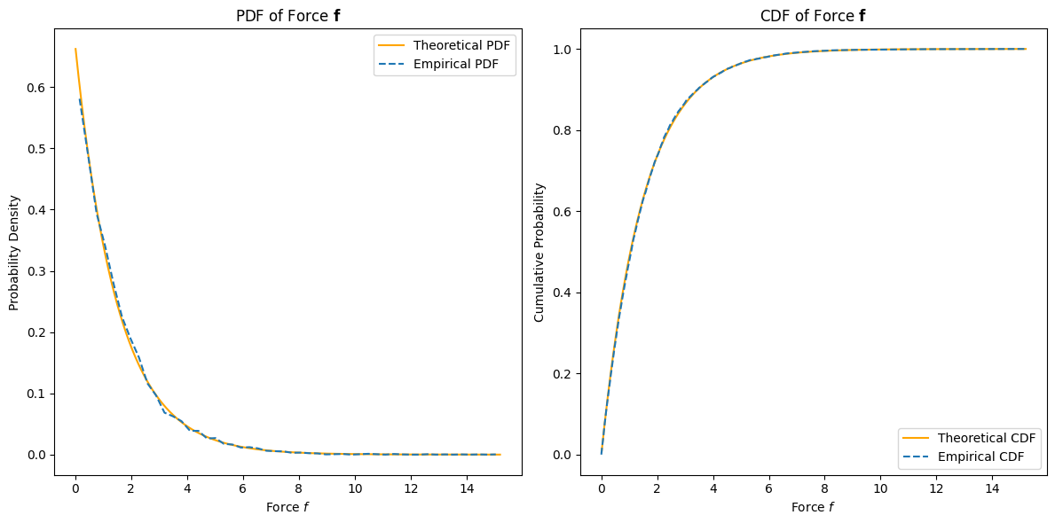
The derived PDF \( p_{\mathbf{f}}(f) \) indicates that the force \( \mathbf{f} \) follows an exponential distribution scaled by the mass \( m \) and the parameter \( \lambda \). This result aligns with the fact that force is linearly related to acceleration by the constant mass \( m \), and since acceleration \( \mathbf{a} \) is exponentially distributed, so is the force \( \mathbf{f} \). The exponential decay in the PDF suggests that higher forces are less likely, consistent with the nature of exponential distributions.

Simulation#

To verify the theoretical result through simulation, we will:

Generate samples of acceleration \( \mathbf{a} \) from an exponential distribution.
Derive the force \( \mathbf{f} \) from \( \mathbf{a} \) using the relation \( \mathbf{f} = m \mathbf{a} \).
Estimate the pdf and cdf from samples of \( \mathbf{f} \).
Plot and compare the empirical cdf and pdf with the theoretical cdf and pdf.

import numpy as np
import matplotlib.pyplot as plt
from scipy.stats import expon

# Parameters
lambda_param = 2  # parameter of the exponential distribution
mass = 3  # mass of the object
num_samples = 10000  # number of samples

# Generate samples of acceleration a
a_samples = np.random.exponential(scale=1/lambda_param, size=num_samples)

# Derive force f from acceleration a
f_samples = mass * a_samples

# Theoretical pdf of force f
def pdf_f(f, lambda_param, mass):
    return (lambda_param / mass) * np.exp(-lambda_param * f / mass) * (f > 0)

# Theoretical cdf of force f
def cdf_f(f, lambda_param, mass):
    return 1 - np.exp(-lambda_param * f / mass)

# Generate values for f for theoretical pdf and cdf
f_values = np.linspace(0.01, np.max(f_samples), 1000)  # start from 0.01 to avoid 0
pdf_f_values = pdf_f(f_values, lambda_param, mass)
cdf_f_values = cdf_f(f_values, lambda_param, mass)

# Empirical pdf estimation using histogram
hist, bin_edges = np.histogram(f_samples, bins=50, density=True)
bin_centers = (bin_edges[:-1] + bin_edges[1:]) / 2

# Remove the value at 0, just for plotting purposes
non_zero_indices = bin_centers > 0
bin_centers = bin_centers[non_zero_indices]
hist = hist[non_zero_indices]

# Empirical cdf estimation
sorted_f_samples = np.sort(f_samples)
empirical_cdf = np.arange(1, num_samples + 1) / num_samples

# Plotting
plt.figure(figsize=(12, 6))

# Plot empirical and theoretical pdf
plt.subplot(1, 2, 1)
plt.plot(f_values, pdf_f_values, label='Theoretical PDF', color='orange')
plt.plot(bin_centers, hist, label='Empirical PDF', linestyle='dashed')
plt.title('PDF of Force $\\mathbf{f}$')
plt.xlabel('Force $f$')
plt.ylabel('Probability Density')
plt.legend()

# Plot empirical and theoretical cdf
plt.subplot(1, 2, 2)
plt.plot(f_values, cdf_f_values, label='Theoretical CDF', color='orange')
plt.plot(sorted_f_samples, empirical_cdf, label='Empirical CDF', linestyle='dashed')
plt.title('CDF of Force $\\mathbf{f}$')
plt.xlabel('Force $f$')
plt.ylabel('Cumulative Probability')
plt.legend()

plt.tight_layout()
plt.show()

_images/ad3f1fe4cc4b5d95a43045b37565faec8c5f030db0f2932efc941886070c8836.png

Methods of computing the pdf of a function of a random variable#

Two methods used to compute the pdf of a function of a random variable include:

Direct method
Leibnitz’s rule

Direct method#

The direct method involves using the known function and the pdf (probability density function) of the original random variable to derive the pdf of the transformed random variable.

APPLICATION. for backpropagation derivation in the training of a neural network.

Example: Linear Transformation#

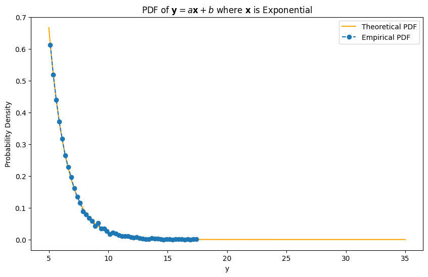
Consider the linear transformation \( \mathbf{y} = a\mathbf{x} + b \) with \( a > 0 \). Our objective is to determine the CDF and PDF of \( \mathbf{y} \) given the CDF and PDF of \( \mathbf{x} \) using the direct method.

CDF of \( \mathbf{y} \)#

The cumulative distribution function (CDF) of \( \mathbf{y} \), denoted as \( F_{\mathbf{y}}(y) \), is defined by:

\[ F_{\mathbf{y}}(y) = P(\mathbf{y} \leq y) \]

Substituting \( \mathbf{y} = a\mathbf{x} + b \) into the inequality, we get:

\[ P(\mathbf{y} \leq y) = P(a \mathbf{x} + b \leq y) \]

To isolate \( \mathbf{x} \), we rearrange the inequality:

\[ P(a \mathbf{x} + b \leq y) = P\left( \mathbf{x} \leq \frac{y - b}{a} \right) \]

This expression corresponds to the CDF of \( \mathbf{x} \), so we can write:

\[ P\left( \mathbf{x} \leq \frac{y - b}{a} \right) = F_{\mathbf{x}}\left( \frac{y - b}{a} \right) \]

PDF of \( \mathbf{y} \)#

To find the probability density function (PDF) of \( \mathbf{y} \), we differentiate the CDF \( F_{\mathbf{y}}(y) \) with respect to \( y \):

\[ p_{\mathbf{y}}(y) = \frac{d}{dy} F_{\mathbf{y}}(y) \]

Using the chain rule, this becomes:

\[ p_{\mathbf{y}}(y) = \frac{d}{dy} F_{\mathbf{x}}\left( \frac{y - b}{a} \right) = p_{\mathbf{x}}\left( \frac{y - b}{a} \right) \cdot \frac{d}{dy} \left( \frac{y - b}{a} \right) \]

The derivative \( \frac{d}{dy} \left( \frac{y - b}{a} \right) \) simplifies to \( \frac{1}{a} \), so we have:

\[ p_{\mathbf{y}}(y) = p_{\mathbf{x}}\left( \frac{y - b}{a} \right) \cdot \frac{1}{a} \]

Thus, the PDF of \( \mathbf{y} \) is given by:

\[ p_{\mathbf{y}}(y) = \frac{1}{a} p_{\mathbf{x}}\left( \frac{y - b}{a} \right) \]

Leibniz’s Rule Method#

Leibniz’s rule is a useful tool for differentiating an integral with respect to a parameter, especially when the limits of integration are functions of that parameter.

The rule is stated as:

\[ \frac{d}{du} \int_{A(u)}^{B(u)} F(u, \xi) \, d\xi = \int_{A(u)}^{B(u)} \frac{\partial F(u, \xi)}{\partial u} \, d\xi + F(u, B(u)) \frac{dB(u)}{du} - F(u, A(u)) \frac{dA(u)}{du} \]

Applying Leibniz’s Rule in the Context of Random Variables#

To illustrate how Leibniz’s rule applies to the transformation of random variables, consider the transformation \( \mathbf{y} = a\mathbf{x} + b \) with \( a \neq 0 \).

The cumulative distribution function (CDF) of \( \mathbf{y} \), \( F_{\mathbf{y}}(y) \), is:

\[ F_{\mathbf{y}}(y) = P(\mathbf{y} \leq y) = P(a \mathbf{x} + b \leq y) = P\left( \mathbf{x} \leq \frac{y - b}{a} \right) = F_{\mathbf{x}}\left( \frac{y - b}{a} \right) \]

This can also be expressed as:

\[ F_{\mathbf{x}}\left( \frac{y - b}{a} \right) = \int_{-\infty}^{(y-b)/a} p_{\mathbf{x}}(\xi) \, d\xi \]

To find the probability density function (PDF) of \( \mathbf{y} \), we differentiate the CDF \( F_{\mathbf{y}}(y) \) with respect to \( y \) using Leibniz’s rule:

\[ \frac{d}{dy} \int_{-\infty}^{(y-b)/a} p_{\mathbf{x}}(\xi) \, d\xi \]

Here, \( u = y \), \( A(y) = -\infty \), and \( B(y) = \frac{y - b}{a} \).

Since \( A(y) \) is a constant (specifically \( -\infty \)), we have \( \frac{dA(y)}{du} = 0 \). For \( B(y) = \frac{y - b}{a} \), the derivative is \( \frac{dB(y)}{dy} = \frac{1}{a} \).

Thus, applying Leibniz’s rule, we get:

\[ \frac{d}{dy} \int_{-\infty}^{(y-b)/a} p_{\mathbf{x}}(\xi) \, d\xi = \int_{-\infty}^{(y-b)/a} \frac{\partial p_{\mathbf{x}}(\xi)}{\partial y} \, d\xi + p_{\mathbf{x}}\left( \frac{y - b}{a} \right) \cdot \frac{1}{a} \]

Since \( p_{\mathbf{x}}(\xi) \) does not explicitly depend on \( y \), the partial derivative \( \frac{\partial p_{\mathbf{x}}(\xi)}{\partial y} = 0 \). Therefore:

\[ \frac{d}{dy} \int_{-\infty}^{(y-b)/a} p_{\mathbf{x}}(\xi) \, d\xi = p_{\mathbf{x}}\left( \frac{y - b}{a} \right) \cdot \frac{1}{a} \]

Thus, the PDF of \( \mathbf{y} \) is:

\[ p_{\mathbf{y}}(y) = \frac{1}{a} p_{\mathbf{x}}\left( \frac{y - b}{a} \right) \]

Handling Negative \( a \)

When \( a < 0 \), the transformation reverses the inequality:

\[ F_{\mathbf{y}}(y) = P(\mathbf{y} \leq y) = P(a \mathbf{x} + b \leq y) = P\left( \mathbf{x} \geq \frac{y - b}{a} \right) \]

Rewriting in terms of the complement:

\[ F_{\mathbf{y}}(y) = 1 - P\left( \mathbf{x} < \frac{y - b}{a} \right) = 1 - \int_{(y-b)/a}^{\infty} p_{\mathbf{x}}(\xi) \, d\xi \]

Differentiating the CDF:

\[ p_{\mathbf{y}}(y) = \frac{d}{dy} \left[ 1 - \int_{(y-b)/a}^{\infty} p_{\mathbf{x}}(\xi) \, d\xi \right] = -\left( -\frac{1}{a} p_{\mathbf{x}}\left( \frac{y - b}{a} \right) \right) = \frac{1}{|a|} p_{\mathbf{x}}\left( \frac{y - b}{a} \right) \]

import numpy as np
import matplotlib.pyplot as plt
from scipy.stats import expon

# Parameters
lambda_param = 2  # parameter of the exponential distribution for x
a = 3  # scaling factor
b = 5  # translation factor
num_samples = 10000  # number of samples

# Generate samples of x from exponential distribution
x_samples = np.random.exponential(scale=1/lambda_param, size=num_samples)

# Derive y from x using y = a*x + b
y_samples = a * x_samples + b

# Theoretical pdf of y
def pdf_y(y, lambda_param, a, b):
    return (lambda_param / a) * np.exp(-lambda_param * (y - b) / a) * (y >= b)

# Generate values for y for theoretical pdf
y_values = np.linspace(b, b + 10 * a, 1000)
pdf_y_values = pdf_y(y_values, lambda_param, a, b)

# Empirical pdf estimation using histogram
hist, bin_edges = np.histogram(y_samples, bins=50, density=True)
bin_centers = (bin_edges[:-1] + bin_edges[1:]) / 2

# Plotting
plt.figure(figsize=(10, 6))

# Plot empirical and theoretical pdf
plt.plot(y_values, pdf_y_values, label='Theoretical PDF', color='orange')
plt.plot(bin_centers, hist, label='Empirical PDF', linestyle='dashed', marker='o')
plt.title('PDF of $\\mathbf{y} = a\\mathbf{x} + b$ where $\\mathbf{x}$ is Exponential')
plt.xlabel('y')
plt.ylabel('Probability Density')
plt.legend()

plt.show()

_images/c895515bce2947ffb9e270e51a44f775cd0d2f7436565786b294d41a6005676b.png

General Case for Multiple Roots#

When the function \( y = g(x) \) has multiple roots \( x_1, x_2, \ldots, x_m \) such that \( y = g(x_1) = g(x_2) = \cdots = g(x_m) \), the probability density function (PDF) of \( y \) includes contributions from each root. The PDF is adjusted for each root by the absolute value of the derivative \( g'(x_i) \) at that root:

\[ p_{\mathbf{y}}(y) = \sum_{i=1}^{m} \frac{p_{\mathbf{x}}(x_i)}{|g'(x_i)|} \]

where \( x_i \) are the roots such that \( g(x_i) = y \), and \( g'(x_i) \) is the derivative of \( g \) evaluated at \( x_i \).

Example with Multiple Roots#

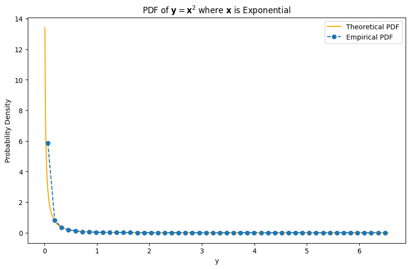
Consider a scenario where the random variable \( \mathbf{y} \) is defined as a function of \( \mathbf{x} \) with multiple roots. Specifically, let’s examine the case where \( \mathbf{y} = \mathbf{x}^2 \).

For a given \( y \), there are two possible values of \( \mathbf{x} \) that satisfy the equation \( y = \mathbf{x}^2 \): \( x_1 = \sqrt{y} \) and \( x_2 = -\sqrt{y} \).

The derivative of \( g(x) = x^2 \) is:

\[ g'(x) = 2x \]

Evaluating the derivative at the roots:

\[ g'(\sqrt{y}) = 2\sqrt{y}, \quad g'(-\sqrt{y}) = -2\sqrt{y} \]

According to the formula for multiple roots, the PDF of \( \mathbf{y} \) is:

\[ p_{\mathbf{y}}(y) = \frac{p_{\mathbf{x}}(x_1)}{|g'(x_1)|} + \frac{p_{\mathbf{x}}(x_2)}{|g'(x_2)|} \]

Substituting the values, the PDF of \( \mathbf{y} \) becomes:

\[ p_{\mathbf{y}}(y) = \frac{p_{\mathbf{x}}(\sqrt{y})}{|2\sqrt{y}|} + \frac{p_{\mathbf{x}}(-\sqrt{y})}{|2\sqrt{y}|} \]

Since \( p_{\mathbf{x}}(\sqrt{y}) = p_{\mathbf{x}}(-\sqrt{y}) \) for symmetric distributions (such as the normal distribution), we obtain:

\[ p_{\mathbf{y}}(y) = \frac{2p_{\mathbf{x}}(\sqrt{y})}{2\sqrt{y}} = \frac{p_{\mathbf{x}}(\sqrt{y})}{\sqrt{y}} \]

This expression is valid for \( y \geq 0 \), and \( p_{\mathbf{y}}(y) = 0 \) for \( y < 0 \).

Specific Distribution of \( \mathbf{x} \)#

Assume \( \mathbf{x} \) follows a standard normal distribution, with the PDF given by:

\[ p_{\mathbf{x}}(x) = \frac{1}{\sqrt{2\pi}} e^{-x^2 / 2} \]

Then, the PDF of \( \mathbf{y} \) (for \( y \geq 0 \)) is:

\[ p_{\mathbf{y}}(y) = \frac{p_{\mathbf{x}}(\sqrt{y})}{\sqrt{y}} = \frac{1}{\sqrt{2\pi}} \frac{e^{-\frac{(\sqrt{y})^2}{2}}}{\sqrt{y}} = \frac{1}{\sqrt{2\pi y}} e^{-y / 2} \]