Power Spectral Density

Power Spectral Density of a Digitally Modulated Signal with Memory

We analyze a bandpass modulated signal \( v(t) \) through its equivalent complex-valued, lowpass signal \( v_{lp}(t) \):

\[ v_{lp}(t) = \sum_{n=-\infty}^{\infty} s_{lp}(t - nT; \vec{I}_n) \]

• \( s_{lp}(t; \vec{I}_n) \) represents one of \( M \) possible lowpass signals based on the information sequence \( \vec{I}_n \).

• The process \( \vec{I}_n = (\ldots, I_{n-2}, I_{n-1}, I_{n}) \) is stationary.

The goal is to determine the power spectral density (PSD) of \( v(t) \).

Autocorrelation of \( v_{lp}(t) \)

The autocorrelation function is given by:

\[ R_{v_{lp}}(t + \tau, t) = \mathbb{E}[v_{lp}(t + \tau)v_{lp}^*(t)] \]

\[ = \sum_{n=-\infty}^{\infty} \sum_{m=-\infty}^{\infty} \mathbb{E}\left[s_{lp}(t + \tau - nT; \vec{I}_n)s_{lp}^*(t - mT; \vec{I}_m)\right] \]

Averaged Autocorrelation

Since \( v_{lp}(t) \) is a cyclostationary process, we average \( R_{v_{lp}}(t + \tau, t) \) over one period \( T \).

The averaged autocorrelation function \( \bar{R}_{v_{lp}}(\tau) \) is:

\[ \bar{R}_{v_{lp}}(\tau) = \frac{1}{T} \sum_{k=-\infty}^{\infty} \sum_{m=-\infty}^{\infty} \int_0^T \mathbb{E}[s_{lp}(t + \tau - mT - kT; \vec{I}_{m+k})s_{lp}^*(t - mT; \vec{I}_m)]\,dt \]

After a variable change \( u = t - mT \):

\[ = \frac{1}{T} \sum_{k=-\infty}^{\infty} \sum_{m=-\infty}^{\infty} \int_{-mT}^{(m-1)T} \mathbb{E}[s_{lp}(u + \tau - kT; \vec{I}_k)s_{lp}^*(u; \vec{I}_0)]\,du \]

Definition of \( g_k(\tau) \)

The function \( g_k(\tau) \) is defined as:

\[ g_k(\tau) = \int_{-\infty}^{\infty} \mathbb{E}\left[ s_{lp}(t + \tau; \vec{I}_k)s_{lp}^*(t; \vec{I}_0)\right] dt \]

which represents the expected autocorrelation between pulses separated by \( k \) symbol periods.

Averaged Autocorrelation in Terms of \( g_k(\tau) \)

Next, the autocorrelation function can be decomposed into a sum of time-shifted versions of \( g_k(\tau) \) as:

\[ \bar{R}_{v_{lp}}(\tau) = \frac{1}{T}\sum_{k=-\infty}^{\infty} g_k(\tau - kT) \]

Power Spectral Density (PSD) of \( v_{lp}(t) \)

The power spectral density, \( S_{v_{lp}}(f) \), is the Fourier transform of \( \bar{R}_{v_{lp}}(\tau) \):

\[ S_{v_{lp}}(f) = \frac{1}{T} \mathcal{F}\left[\sum_{k=-\infty}^{\infty} g_k(\tau - kT)\right] \]

By applying the Fourier transform of time-shifted signals:

\[ S_{v_{lp}}(f) = \frac{1}{T}\sum_{k=-\infty}^{\infty} G_k(f)e^{-j2\pi kfT} \]

where \( G_k(f) \) is the Fourier transform of \( g_k(\tau) \).

Expression for \( G_k(f) \)

The quantity \( G_k(f) \) is derived as:

\[ G_k(f) = \mathcal{F}\left[\int_{-\infty}^{\infty}\mathbb{E}[s_{lp}(t + \tau; \vec{I}_k)s_{lp}^*(t; \vec{I}_0)]dt\right] \]

Expanding:

\[ G_k(f) = \mathbb{E}\left[\int_{-\infty}^{\infty}\int_{-\infty}^{\infty} s_{lp}(t + \tau; \vec{I}_k)e^{-j2\pi f(t+\tau)} s_{lp}^*(t; \vec{I}_0)e^{j2\pi f t} dt d\tau\right] \]

which simplifies to:

\[ G_k(f) = \mathbb{E}[S_{lp}(f; \vec{I}_k)S_{lp}^*(f; \vec{I}_0)] \]

where \( S_{lp}(f; \vec{I}_k) \) and \( S_{lp}(f; \vec{I}_0) \) are the Fourier transforms of \( s_{lp}(t; \vec{I}_k) \) and \( s_{lp}(t; \vec{I}_0) \).

Relationship of \( G_k(f) \)

We have:

\[ G_0(f) = \mathbb{E}\left[|S_{lp}(f; \vec{I}_0)|^2\right] \]

where \( G_0(f) \) is real.

For \( k \geq 1 \), \( G_{-k}(f) = G_k^*(f) \).

We define:

\[ G'_k(f) = G_k(f) - G_0(f) \]

From this definition:

\[ G'_{-k}(f) = G'_k(f)^*, \quad G'_0(f) = 0 \]

This redefinition centers the spectral components around \( G_0(f) \) and introduces symmetry properties.

Final PSD Expression

Using these definitions, the PSD \( S_{v_{lp}}(f) \) becomes:

\[ S_{v_{lp}}(f) = \frac{1}{T}\sum_{k=-\infty}^{\infty}[G_k(f) - G_0(f)]e^{-j2\pi kfT} + \frac{1}{T}\sum_{k=-\infty}^{\infty}G_0(f)e^{-j2\pi kfT} \]

Rearranging:

\[ = \frac{1}{T}\sum_{k=-\infty}^{\infty}G'_k(f)e^{-j2\pi kfT} + \frac{1}{T^2}\sum_{k=-\infty}^{\infty}G_0\left(\frac{k}{T}\right)\delta\left(f - \frac{k}{T}\right) \]

Continuous and Discrete Components

By leveraging symmetry properties and Fourier properties:

\[ \boxed{ S_{v_{lp}}(f) = S_{v_{lp}}^{(c)}(f) + S_{v_{lp}}^{(d)}(f) } \]

where:

• Continuous Component:

\[ S_{v_{lp}}^{(c)}(f) = \frac{2}{T}\text{Re}\left[\sum_{k=1}^{\infty}G'_k(f)e^{-j2\pi kfT}\right] \]

• Discrete Component:

\[ S_{v_{lp}}^{(d)}(f) = \frac{1}{T^2}\sum_{k=-\infty}^{\infty}G_0\left(\frac{k}{T}\right)\delta\left(f - \frac{k}{T}\right) \]

Power Spectral Density of Linearly Modulated Signals

We consider Linearly Modulated Signals, which encompasses modulation schemes like ASK, PSK, and QAM.

For linearly modulated signals, the lowpass equivalent of the modulated signal \( v_{lp}(t) \) is:

\[ v_{lp}(t) = \sum_{n=-\infty}^{\infty} I_n g(t - nT) \]

where:

• \( I_n \): Stationary information component (random symbols, the last component of the sequence \(\vec{I}_n\) considered previously.

• \( g(t) \): Basic modulation pulse (e.g., rectangular pulse).

• \( T \): Symbol period.

Correspondence with the General Model

Comparing with the general form of \( v_{lp}(t) \) above, we get:

\[ s_{lp}(t, \vec{I}_n) = I_n g(t) \]

Thus, the signal consists of symbols \( I_n \) multiplied by a common base pulse \( g(t) \).

Derivation of \( G_k(f) \)

Recall from previous equations:

\[ G_k(f) = \mathbb{E}\left[S_{lp}(f; \vec{I}_k)S_{lp}^*(f; \vec{I}_0)\right] \]

Now, given \( s_{lp}(t, \vec{I}_n) = I_n g(t)\), the Fourier transform of \( s_{lp}(t, \vec{I}_n) \) is:

\[ S_{lp}(f; \vec{I}_n) = I_n G(f) \]

where \( G(f) \) is the Fourier transform of \( g(t) \).

So:

\[ G_k(f) = \mathbb{E}\left[I_k I_0^* |G(f)|^2\right] \]

The expectation applies only to \( I_k \) and \( I_0 \):

\[ G_k(f) = R_{II}(k)|G(f)|^2 \]

where:

• \( R_{II}(k) \) is the autocorrelation function of the information sequence \( \{I_n\} \).

• \( |G(f)|^2 \) is the magnitude squared of the Fourier transform of the modulation pulse \( g(t) \).

Derivation of \( S_{v_{lp}}(f) \)

The PSD of \( v_{lp}(t) \) is:

\[ S_{v_{lp}}(f) = \frac{1}{T}\sum_{k=-\infty}^{\infty} G_k(f)e^{-j2\pi kfT} \]

Substituting \( G_k(f) \):

\[ S_{v_{lp}}(f) = \frac{1}{T}\sum_{k=-\infty}^{\infty} \left[R_{II}(k)|G(f)|^2\right]e^{-j2\pi kfT} \]

Factor \( |G(f)|^2 \) out:

\[ S_{v_{lp}}(f) = \frac{|G(f)|^2}{T}\sum_{k=-\infty}^{\infty} R_{II}(k)e^{-j2\pi kfT} \]

Recognizing the summation as the discrete-time Fourier transform (DTFT) of the autocorrelation function \( R_{II}(k) \), we define:

\[ S_I(f) = \sum_{k=-\infty}^{\infty} R_{II}(k)e^{-j2\pi kfT} \]

Thus, the power spectral density of \( v_{lp}(t) \) is:

\[ \boxed{ S_{v_{lp}}(f) = \frac{|G(f)|^2}{T}S_I(f) } \]

where

• \( |G(f)|^2 \) reflects the energy distribution of the base pulse shape \( g(t) \).

• \( S_I(f) \) characterizes the spectral properties of the symbol sequence \( I_n \).

Precoding

Precoding introduces memory into the transmitted symbols by defining a new sequence \( \{J_n\} \) from the original sequence \( \{I_n\} \).

The general precoding can be expressed as

\[ \boxed{ J_n = \sum_{k=0}^{L} \alpha_k I_{n-k} } \]

where:

• \( L \): Length of the memory in the precoder.

• \( \alpha_k \): Coefficients that determine the contribution of past symbols \( I_{n-k} \) to the current precoded symbol \( J_n \).

When \( L = 1 \) and \( \alpha_1 = \alpha \), the simple precoder becomes:

\[ J_n = I_n + \alpha I_{n-1} \]

By adjusting \( \alpha \), the correlation properties of the signal are modified, which in turn changes the PSD.

Modulated Waveform After Precoding

After applying the precoding process, the transmitted waveform becomes:

\[ v_{lp}(t) = \sum_{k=-\infty}^{\infty} J_k g(t - kT) \]

We can see that:

• Each symbol \( J_k \) is convolved with the base pulse \( g(t) \).

• The resulting waveform inherits the correlation properties introduced by the precoding.

PSD of the Precoded Signal

Since the precoding is linear, the PSD of the precoded signal can be derived similarly to the original PSD:

\[ S_{v_{lp}}(f) = \frac{1}{T}|G(f)|^2 \left| \sum_{k=0}^{L}\alpha_k e^{-j2\pi kfT}\right|^2 S_I(f) \]

where:

• \( |G(f)|^2 \): Spectrum of the base pulse \( g(t) \).

• \( S_I(f) \): PSD of the original information sequence.

The additional factor:

\[ \left|\sum_{k=0}^{L}\alpha_k e^{-j2\pi kfT}\right|^2 \]

reflects the impact of the precoding on the PSD. By choosing different values of \( \alpha_k \), we can control the correlation of symbols and, consequently, the spectral characteristics of the signal.

Practical Significance

• Spectral Efficiency: Adjusting \( \alpha_k \) can minimize spectral side lobes, making transmissions more bandwidth-efficient.

• ISI Mitigation: Precoding can help shape the spectrum to reduce intersymbol interference in practical communication systems.

Example: Binary Communication System

Given an information sequence:

• \( I_n = \pm 1 \) with equal probability (binary sequence).

• Symbols are independent and identically distributed.

Pulse Shape

The information stream linearly modulates a rectangular pulse defined by:

\[ g(t) = \Pi\left(\frac{t}{T}\right) \]

where \( \Pi(x) \) is a rectangular function, which equals 1 for \(|x| \leq 0.5\) and 0 otherwise.

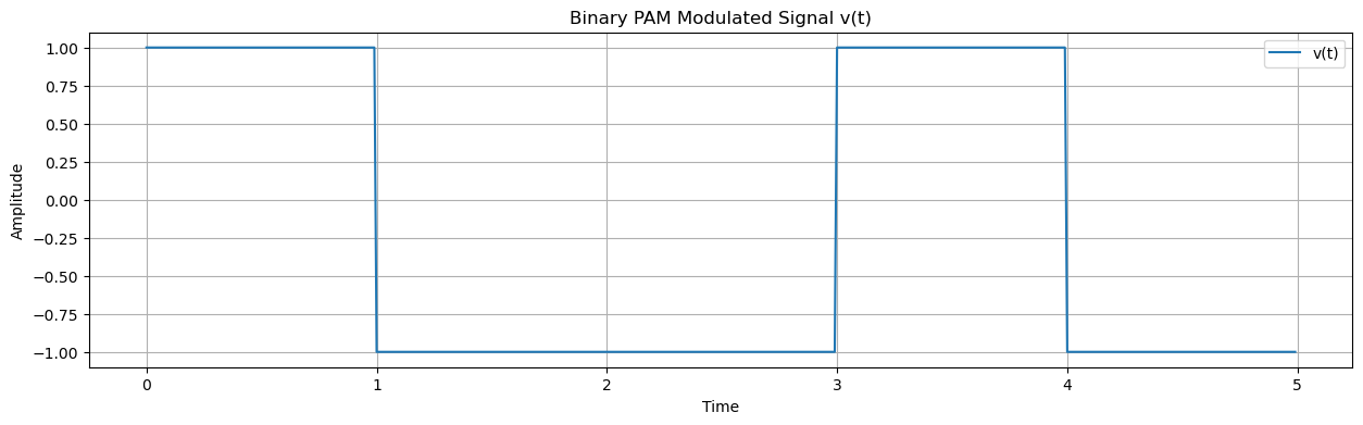
Generated Modulated Signal

The modulated signal is:

\[ v(t) = \sum_{k=-\infty}^{\infty} I_k g(t - kT) \]

This represents a binary PAM waveform modulated by rectangular pulses.

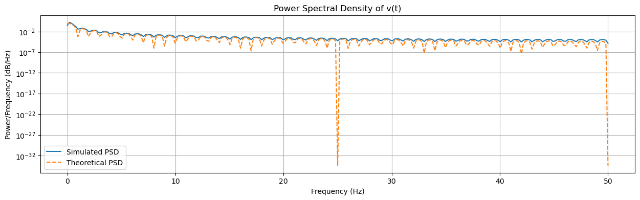
Power Spectral Density (PSD)

The PSD of the modulated signal is given by:

\[ S_{v}(f) = \frac{1}{T}|T\text{sinc}(Tf)|^2 S_I(f) \]

Autocorrelation of \( I_n \)

Since the symbols are independent and identically distributed:

\[ R_{II}(k) = \mathbb{E}[I_{n+k}I_n] \]

Note that \(I_n\) is real-valued, so we do not need to use \(I_n^*\) in \(R_{II}(k)\). We further have:

• For \( k = 0 \): \( R_{II}(0) = 1 \) (variance of binary \(\pm 1\) symbols is 1).

• For \( k \ne 0 \): \( R_{II}(k) = 0 \) due to independence.

Thus:

\[ S_I(f) = \sum_{k=-\infty}^{\infty} R_{II}(k)e^{-j2\pi kfT} = 1 \]

So the PSD becomes:

\[ \boxed{ S_{v}(f) = T\text{sinc}^2(Tf) } \]

Precoding with Memory

A precoder is applied to shape the spectrum:

\[ J_n = I_n + \alpha I_{n-1} \]

This introduces correlation between consecutive symbols, affecting the spectrum.

PSD with Precoding

The resulting PSD with this first-order precoding is:

\[ S_{v}(f) = T\text{sinc}^2(Tf)\left|1 + \alpha e^{-j2\pi fT}\right|^2 \]

Expanding:

\[ S_{v}(f) = T\text{sinc}^2(Tf)\left(1 + \alpha^2 + 2\alpha\cos(2\pi fT)\right) \]

Special Case: \(\alpha = 1\)

If:

\[ \alpha = 1 \]

Then the PSD exhibits a spectral null at:

\[ f = \frac{1}{2T} \]

This null occurs regardless of the shape of \( g(t) \), indicating that precoding can shape the spectrum independently of the pulse shape.

import numpy as np
import matplotlib.pyplot as plt
from scipy.signal import welch

# Parameters
T = 1  # Symbol duration
Fs = 100  # Sampling frequency
Ts = 1 / Fs  # Sampling period
N = 100  # Number of symbols

# Generate random binary sequence I_n
I_n = np.random.choice([-1, 1], size=N)

# Time vector
t = np.arange(-T/2, T/2, Ts)

# Define rectangular pulse g(t)
g_t = np.where((t >= -T/2) & (t < T/2), 1, 0)

# Generate modulated signal v(t)
time_axis = np.arange(0, N*T, Ts)
v_t = np.zeros_like(time_axis)

for k in range(N):
    v_t[k * Fs: (k + 1) * Fs] += I_n[k] * g_t

# Compute PSD using Welch's method
f, Pxx = welch(v_t, fs=Fs, nperseg=512)

# Theoretical PSD S_v(f) = T sinc^2(Tf)
S_v_theoretical = T * (np.sinc(f * T))**2

# Plot modulated signal v(t)
plt.figure(figsize=(15, 4))
plt.plot(time_axis[:5*Fs], v_t[:5*Fs], label="v(t)")
plt.title("Binary PAM Modulated Signal v(t)")
plt.xlabel("Time")
plt.ylabel("Amplitude")
plt.legend()
plt.grid()
plt.show()

# Plot PSD comparison
plt.figure(figsize=(15, 4))
plt.semilogy(f, Pxx, label="Simulated PSD")
plt.semilogy(f, S_v_theoretical, '--', label="Theoretical PSD")
plt.title("Power Spectral Density of v(t)")
plt.xlabel("Frequency (Hz)")
plt.ylabel("Power/Frequency (dB/Hz)")
plt.legend()
plt.grid()
plt.show()

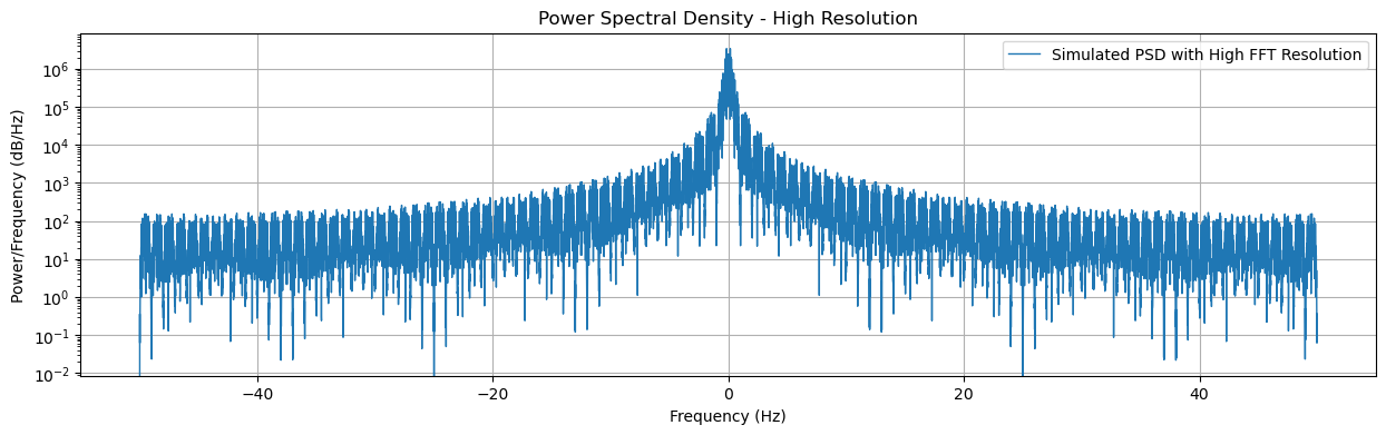
# Increase FFT size for better resolution
fft_size = 8192  # Large FFT for high frequency resolution

# Compute PSD using direct FFT
V_f = np.fft.fftshift(np.fft.fft(v_t, n=fft_size))  # Compute FFT and shift zero freq to center
freqs = np.fft.fftshift(np.fft.fftfreq(fft_size, d=Ts))  # Compute frequency axis

# Compute magnitude squared (PSD estimate)
PSD_direct = np.abs(V_f) ** 2

# Create a new plot for better resolution
plt.figure(figsize=(15, 4))
plt.semilogy(freqs, PSD_direct, label="Simulated PSD with High FFT Resolution", linewidth=1)

plt.title("Power Spectral Density - High Resolution")
plt.xlabel("Frequency (Hz)")
plt.ylabel("Power/Frequency (dB/Hz)")
plt.legend()
plt.grid()
plt.show()