Signal Space#
The idea of an orthonormal basis is analogous to the alphabet in language, providing the foundational elements needed to construct more complex entities.
Alphabet and Vector Space Analogy:
The 26 letters of the English alphabet are the fundamental building blocks used to form all words and vocabularies. Similarly, an orthonormal basis is a set of fundamental vectors that spans the entire vector space.
Just as any word can be constructed by combining letters in different proportions, any vector in a space can be expressed as a unique linear combination of orthonormal basis vectors.
This analogy highlights the simplicity and universality of orthonormal bases: they reduce complexity by defining a minimal set of independent “building blocks” for representing elements in a vector space.
Signal Space Analogy:
In communication and signal processing, we often work within a signal space, where signals are represented as vectors. For specific tasks, such as modulation, it is sufficient to define an orthonormal signal basis for that space.
Just as an orthonormal basis in a vector space allows any vector to be uniquely represented, an orthonormal signal basis allows any signal to be uniquely decomposed into a weighted combination of these basis signals.
For example, in modulation schemes like QAM or PSK, orthonormal basis functions (e.g., sine and cosine waves) serve as the building blocks for representing transmitted signals.
Why This Works:
Simplicity: Orthonormal bases simplify projections, decompositions, and computations due to their independence and normalization properties.
Uniqueness: Each vector or signal has a unique representation in terms of the orthonormal basis, ensuring clarity and efficiency.
Efficiency: In signal processing, orthonormal bases eliminate redundancy and provide compact representations (e.g., Fourier or wavelet transforms).
In summary, just as the alphabet provides the fundamental structure for constructing meaningful language, an orthonormal basis serves as the foundational framework for representing, analyzing, and processing elements in vector and signal spaces.
Vector Space#
We introduce key concepts related to vectors in \(n\)-dimensional space.
Vector Representation#
Vector Space Concepts
A vector \( \vec{v} \) in an \( n \)-dimensional space is defined by its \( n \) components \( v_1, v_2, ..., v_n \). It is often represented as a column vector, i.e., \( \vec{v} = [v_1, v_2, ..., v_n]^T \), where \( A^T \) denotes the transpose of a matrix \( A \).
Additional Concepts
Two vectors are said to be orthogonal if their inner product is zero, i.e., \( \langle \vec{v}_1, \vec{v}_2 \rangle = 0 \).
A set of \( m \) vectors is linearly independent if no vector can be expressed as a linear combination of the others.
Definition: Inner Product of Two Vectors#
The inner product of two \( n \)-dimensional vectors \( \vec{v}_1 = [v_{11}, v_{12}, ..., v_{1n}]^T \) and \( \vec{v}_2 = [v_{21}, v_{22}, ..., v_{2n}]^T \) is defined as:
where, \( A^H \) (the Hermitian transpose) refers to the transpose of \( A \) followed by conjugating its elements.
Representing Vectors as Linear Combinations#
A vector can be expressed as a linear combination of orthonormal basis vectors \( \vec{e}_i \), where \( i = 1, 2, ..., n \):
where:
Each \( \vec{e}_i \) is a unit vector (i.e., it has a length of 1).
\( v_i \) is the projection of \( \vec{v} \) onto \( \vec{e}_i \), computed as \( v_i = \langle \vec{v}, \vec{e}_i \rangle \).
Orthonormality#
Definition: Orthogonality of Vectors#
Two vectors \( \vec{v}_1 \) and \( \vec{v}_2 \) are orthogonal if their inner product equals zero:
More generally, a set of \( m \) vectors \( \vec{v}_1, \vec{v}_2, ..., \vec{v}_m \) is orthogonal if:
Definition: Vector Norm#
The norm of a vector \( \vec{v} \), denoted \( \| \vec{v} \| \), is defined as:
This represents the length of the vector in \( n \)-dimensional space.
Definition of Orthonormality#
Orthonormality is a property of a set of vectors in a vector space that combines orthogonality and normalization:
Orthogonality: The vectors in the set are pairwise orthogonal. This means that for any two distinct vectors \( \vec{v}_i \) and \( \vec{v}_j \) in the set, their inner product is zero:
\[ \langle \vec{v}_i, \vec{v}_j \rangle = 0 \quad \text{for } i \neq j. \]Normalization: Each vector in the set has unit length, i.e., its norm (or magnitude) is 1:
\[ \|\vec{v}_i\| = \sqrt{\langle \vec{v}_i, \vec{v}_i \rangle} = 1. \]
Key Properties of Orthonormal Sets
Simplicity of Representation: Any vector in the space can be represented as a linear combination of the orthonormal vectors.
Independence: An orthonormal set of vectors is linearly independent.
Example of Orthonormal Vectors in 3D Cartesian Space
In 3D space, the standard basis vectors are:
These vectors are orthonormal because:
Orthogonality: The dot product of any pair of distinct vectors is zero:
\[ \langle \vec{e}_1, \vec{e}_2 \rangle = 0, \quad \langle \vec{e}_2, \vec{e}_3 \rangle = 0, \quad \langle \vec{e}_1, \vec{e}_3 \rangle = 0. \]Normalization: Each vector has unit length:
\[ \|\vec{e}_1\| = 1, \quad \|\vec{e}_2\| = 1, \quad \|\vec{e}_3\| = 1. \]
These vectors form the standard orthonormal basis for 3D Cartesian space.
Python Simulation#
import numpy as np
import matplotlib.pyplot as plt
from mpl_toolkits.mplot3d import Axes3D
# Define the orthonormal basis vectors in 3D Cartesian space
# These are unit vectors along the x, y, and z axes
e1 = np.array([1, 0, 0]) # x-axis unit vector
e2 = np.array([0, 1, 0]) # y-axis unit vector
e3 = np.array([0, 0, 1]) # z-axis unit vector
# Generate a random vector v in 3D space
# The vector v_sim represents an arbitrary vector
v_sim = 5 * np.random.rand(3) # Random vector scaled to have components in [0, 5]
# Calculate the projections (coefficients) of v onto the orthonormal basis vectors
# Each coefficient represents the contribution of the corresponding basis vector
v1 = np.dot(v_sim, e1) # Projection of v onto e1
v2 = np.dot(v_sim, e2) # Projection of v onto e2
v3 = np.dot(v_sim, e3) # Projection of v onto e3
# Reconstruct the vector v as a linear combination of the orthonormal basis vectors
# The linear combination verifies that the original vector can be expressed
# entirely in terms of the orthonormal basis
v_reconstructed = v1 * e1 + v2 * e2 + v3 * e3
# Display the original and reconstructed vectors to verify they are identical
print("Original vector v:")
print(v_sim)
print("Reconstructed vector from orthonormal basis:")
print(v_reconstructed)
# Plot the original and reconstructed vectors, along with the orthonormal basis vectors
fig = plt.figure(figsize=(4, 4))
ax = fig.add_subplot(111, projection='3d')
# Plot the original vector in blue
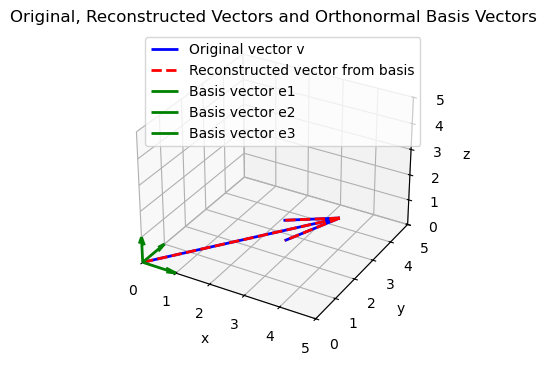
ax.quiver(0, 0, 0, v_sim[0], v_sim[1], v_sim[2], color='b', linewidth=2, label='Original vector v')
# Plot the reconstructed vector in red (dashed line)
ax.quiver(0, 0, 0, v_reconstructed[0], v_reconstructed[1], v_reconstructed[2],
color='r', linestyle='dashed', linewidth=2, label='Reconstructed vector from basis')
# Plot the orthonormal basis vectors in green
ax.quiver(0, 0, 0, e1[0], e1[1], e1[2], color='g', linewidth=2, label='Basis vector e1')
ax.quiver(0, 0, 0, e2[0], e2[1], e2[2], color='g', linewidth=2, label='Basis vector e2')
ax.quiver(0, 0, 0, e3[0], e3[1], e3[2], color='g', linewidth=2, label='Basis vector e3')
# Finalize the plot
ax.set_xlim([0, 5])
ax.set_ylim([0, 5])
ax.set_zlim([0, 5])
ax.set_xlabel('x')
ax.set_ylabel('y')
ax.set_zlabel('z')
ax.set_title('Original, Reconstructed Vectors and Orthonormal Basis Vectors')
ax.legend()
plt.grid()
plt.show()
Original vector v:
[3.42715791 4.15348269 0.22169592]
Reconstructed vector from orthonormal basis:
[3.42715791 4.15348269 0.22169592]
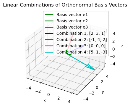
# Example of linear combinations of the orthonormal basis vectors
# Linear combination coefficients
coefficients = [
    [2, 3, 1],  # Example 1: A specific linear combination
    [-1, 4, 2],  # Example 2: A linear combination with negative and positive coefficients
    [0, 0, 0],   # Example 3: A trivial combination (zero vector)
    [5, 1, -3]   # Example 4: A mix with a negative coefficient
]

# Generate the vectors from the linear combinations
linear_combination_vectors = [c[0]*e1 + c[1]*e2 + c[2]*e3 for c in coefficients]

# Display the coefficients and corresponding vectors
print("\nLinear Combination Examples:")
for i, (c, vec) in enumerate(zip(coefficients, linear_combination_vectors), start=1):
    print(f"Combination {i}: Coefficients {c} -> Vector {vec}")

# Plot the linear combination vectors alongside the basis vectors
fig = plt.figure(figsize=(4, 4))
ax = fig.add_subplot(111, projection='3d')

# Plot the orthonormal basis vectors in green
ax.quiver(0, 0, 0, e1[0], e1[1], e1[2], color='g', linewidth=2, label='Basis vector e1')
ax.quiver(0, 0, 0, e2[0], e2[1], e2[2], color='g', linewidth=2, label='Basis vector e2')
ax.quiver(0, 0, 0, e3[0], e3[1], e3[2], color='g', linewidth=2, label='Basis vector e3')

# Plot each linear combination vector in a different color
colors = ['b', 'r', 'm', 'c']  # Colors for different linear combinations
for i, vec in enumerate(linear_combination_vectors):
    ax.quiver(0, 0, 0, vec[0], vec[1], vec[2], color=colors[i % len(colors)], linewidth=2,
              label=f'Combination {i+1}: {coefficients[i]}')

# Finalize the plot
ax.set_xlim([-5, 5])
ax.set_ylim([-5, 5])
ax.set_zlim([-5, 5])
ax.set_xlabel('x')
ax.set_ylabel('y')
ax.set_zlabel('z')
ax.set_title('Linear Combinations of Orthonormal Basis Vectors')
ax.legend()
plt.grid()
plt.show()
Linear Combination Examples:
Combination 1: Coefficients [2, 3, 1] -> Vector [2 3 1]
Combination 2: Coefficients [-1, 4, 2] -> Vector [-1  4  2]
Combination 3: Coefficients [0, 0, 0] -> Vector [0 0 0]
Combination 4: Coefficients [5, 1, -3] -> Vector [ 5  1 -3]
# Verify orthonormality of the set {e1, e2, e3}

# Check orthogonality: Dot product of distinct basis vectors should be zero
orthogonality_checks = {
    "e1 · e2": np.dot(e1, e2),
    "e2 · e3": np.dot(e2, e3),
    "e1 · e3": np.dot(e1, e3),
}

print("Orthogonality checks (dot products between distinct basis vectors):")
for pair, result in orthogonality_checks.items():
    print(f"{pair} = {result:.2f}")

# Check normalization: Norm of each basis vector should be 1
normalization_checks = {
    "||e1||": np.linalg.norm(e1),
    "||e2||": np.linalg.norm(e2),
    "||e3||": np.linalg.norm(e3),
}

print("\nNormalization checks (norms of each basis vector):")
for vec, norm in normalization_checks.items():
    print(f"{vec} = {norm:.2f}")
Orthogonality checks (dot products between distinct basis vectors):
e1 · e2 = 0.00
e2 · e3 = 0.00
e1 · e3 = 0.00

Normalization checks (norms of each basis vector):
||e1|| = 1.00
||e2|| = 1.00
||e3|| = 1.00
Gram-Schmidt Orthogonalization Process#
The Gram-Schmidt process is a method for constructing a set of orthonormal vectors from a set of \( n \)-dimensional vectors \( \vec{v}_i \), where \( 1 \leq i \leq m \). This procedure ensures that the resulting vectors are both orthogonal to each other and normalized to unit length.
Step 1: Normalize the First Vector#
Start by selecting the first vector \( \vec{v}_1 \) from the set. Normalize its length to obtain the first orthonormal vector \( \vec{u}_1 \):
Step 2: Orthogonalize the Second Vector#
Next, take the second vector \( \vec{v}_2 \) and subtract its projection onto \( \vec{u}_1 \) to make it orthogonal to \( \vec{u}_1 \):
Normalize this result to obtain the second orthonormal vector \( \vec{u}_2 \):
Step 3: Orthogonalize Subsequent Vectors#
For the third vector \( \vec{v}_3 \), subtract its projections onto both \( \vec{u}_1 \) and \( \vec{u}_2 \):
Normalize this to get the third orthonormal vector \( \vec{u}_3 \):
Iterative Step: Repeat for All Remaining Vectors#
Continue this process for all subsequent vectors \( \vec{v}_i \), subtracting their projections onto all previously computed orthonormal vectors \( \vec{u}_1, \vec{u}_2, ..., \vec{u}_{i-1} \):
Normalize to obtain the orthonormal vector \( \vec{u}_i \):
Orthonormal Vector Set
By following this procedure, you construct a set of \( N \) orthonormal vectors, where \( N \leq \min(m, n) \). These vectors form an orthonormal basis for the subspace spanned by the original set of vectors.
Python Example#
Example Description#
Input Parameters:
\( m \): Number of input vectors.
\( n \): Dimension of the vectors.
Random Vector Generation:
A matrix \( V \) of size \( n \times m \) is created, where each column represents a random vector:
\[ V = [\vec{v}_1, \vec{v}_2, \dots, \vec{v}_m], \quad V \in \mathbb{R}^{n \times m}. \]
Gram-Schmidt Process for Orthonormalization:
Step 1: Normalize \( \vec{v}_1 \):
\[ \vec{u}_1 = \frac{\vec{v}_1}{\|\vec{v}_1\|} \]Step 2: Orthogonalize \( \vec{v}_2 \):
\[ \text{proj}_{\vec{u}_1}(\vec{v}_2) = \langle \vec{v}_2, \vec{u}_1 \rangle \vec{u}_1 \]\[ \vec{v}_2' = \vec{v}_2 - \text{proj}_{\vec{u}_1}(\vec{v}_2) \]Normalize to get \( \vec{u}_2 \):
\[ \vec{u}_2 = \frac{\vec{v}_2'}{\|\vec{v}_2'\|} \]Step 3: Orthogonalize \( \vec{v}_3 \):
\[ \text{proj}_{\vec{u}_1}(\vec{v}_3) = \langle \vec{v}_3, \vec{u}_1 \rangle \vec{u}_1, \quad \text{proj}_{\vec{u}_2}(\vec{v}_3) = \langle \vec{v}_3, \vec{u}_2 \rangle \vec{u}_2 \]\[ \vec{v}_3' = \vec{v}_3 - \text{proj}_{\vec{u}_1}(\vec{v}_3) - \text{proj}_{\vec{u}_2}(\vec{v}_3) \]Normalize to get \( \vec{u}_3 \):
\[ \vec{u}_3 = \frac{\vec{v}_3'}{\|\vec{v}_3'\|} \]
Output:
An orthonormal set \( U \):
\[ U = \{\vec{u}_1, \vec{u}_2, \vec{u}_3\}. \]
The Gram-Schmidt process stops at 3 vectors because the dimension of the space (\(n = 3\)) limits the number of mutually orthonormal vectors that can be formed.
import numpy as np
import matplotlib.pyplot as plt
# Parameters
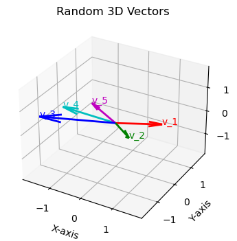
m = 5 # Number of vectors
n = 3 # Dimension of vectors
# Generate a set of random vectors V = [v1, v2, ..., vm]
V = np.random.randn(n, m)
# Plot the random vectors
fig_random = plt.figure(figsize=(4, 4))
ax_random = fig_random.add_subplot(111, projection='3d')
colors = ['r', 'g', 'b', 'c', 'm'] # Colors for plotting
# Plot each random vector
for i in range(m):
ax_random.quiver(0, 0, 0, V[0, i], V[1, i], V[2, i], color=colors[i % len(colors)], linewidth=2)
ax_random.text(V[0, i], V[1, i], V[2, i], f'v_{i+1}', fontsize=10, color=colors[i % len(colors)])
# Configure the random vectors plot
ax_random.set_xlim([-np.max(np.abs(V)), np.max(np.abs(V))])
ax_random.set_ylim([-np.max(np.abs(V)), np.max(np.abs(V))])
ax_random.set_zlim([-np.max(np.abs(V)), np.max(np.abs(V))])
ax_random.set_xlabel('X-axis')
ax_random.set_ylabel('Y-axis')
ax_random.set_zlabel('Z-axis')
ax_random.set_title('Random 3D Vectors')
plt.grid()
plt.show()
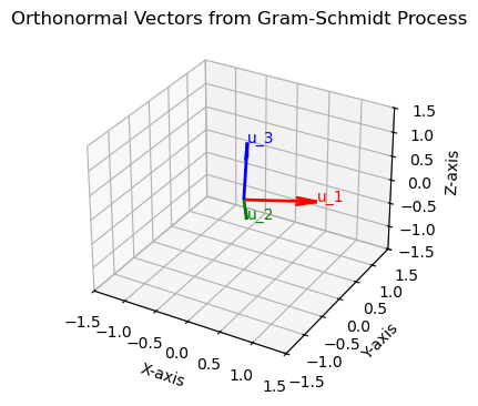
# Gram-Schmidt Process
U = np.zeros((n, n)) # Orthonormal basis vectors (only n can be orthonormal in n-dimensional space)
# Normalize the first vector
U[:, 0] = V[:, 0] / np.linalg.norm(V[:, 0])
# Orthogonalize and normalize remaining vectors
for i in range(1, n):
orthogonal = V[:, i]
for j in range(i):
orthogonal -= np.dot(U[:, j], V[:, i]) * U[:, j] # Subtract projection onto previous basis vectors
U[:, i] = orthogonal / np.linalg.norm(orthogonal)
# Plot the orthonormal vectors
fig_orthonormal = plt.figure(figsize=(4, 4))
ax_orthonormal = fig_orthonormal.add_subplot(111, projection='3d')
colors = ['r', 'g', 'b'] # Colors for orthonormal vectors
# Plot each orthonormal vector
for i in range(n):
ax_orthonormal.quiver(0, 0, 0, U[0, i], U[1, i], U[2, i], color=colors[i % len(colors)], linewidth=2)
ax_orthonormal.text(U[0, i], U[1, i], U[2, i], f'u_{i+1}', fontsize=10, color=colors[i % len(colors)])
# Configure the orthonormal vectors plot
ax_orthonormal.set_xlim([-1.5, 1.5])
ax_orthonormal.set_ylim([-1.5, 1.5])
ax_orthonormal.set_zlim([-1.5, 1.5])
ax_orthonormal.set_xlabel('X-axis')
ax_orthonormal.set_ylabel('Y-axis')
ax_orthonormal.set_zlabel('Z-axis')
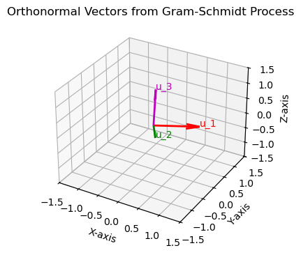
ax_orthonormal.set_title('Orthonormal Vectors from Gram-Schmidt Process')
plt.grid()
plt.show()
# Threshold for considering a value as zero
threshold = 1e-10

# Check orthogonality: Dot products between distinct vectors should be zero
orthogonality_results = np.zeros((n, n))  # Matrix to store dot products
for i in range(n):
    for j in range(n):
        dot_product = np.dot(U[:, i], U[:, j])
        orthogonality_results[i, j] = dot_product if abs(dot_product) >= threshold else 0.0

# Check normalization: Norms of each vector should be 1
normalization_results = [np.linalg.norm(U[:, i]) for i in range(3)]
normalization_results = [norm if abs(norm - 1) >= threshold else 1.0 for norm in normalization_results]

# Display results
print("Orthogonality check (dot product matrix):")
print(orthogonality_results)

print("\nNormalization check (vector norms):")
for i, norm in enumerate(normalization_results):
    print(f"||u_{i+1}|| = {norm:.6f}")
Orthogonality check (dot product matrix):
[[1. 0. 0.]
 [0. 1. 0.]
 [0. 0. 1.]]

Normalization check (vector norms):
||u_1|| = 1.000000
||u_2|| = 1.000000
||u_3|| = 1.000000
Why The Process Stops at 3 Vectors
Dimension of the Space:
In a 3-dimensional space (\(n = 3\)), at most 3 orthonormal vectors can exist, as they must span the entire space.
If you attempt to add a fourth vector, it will always lie in the subspace spanned by the first three vectors, making it impossible to orthogonalize it further.
Rank of the Matrix \( V \):
The random matrix \( V \) has dimensions \( n \times m \) (3 rows, 5 columns). However, the rank of \( V \) cannot exceed \( n = 3 \) because there are only 3 linearly independent directions in a 3D space.
Therefore, only 3 orthonormal vectors can be generated.
Using \( \vec{v}_5 \) Instead of \( \vec{v}_3 \)#
We can use \( \vec{v}_5 \) (or any other vector from the input set \( V \)) instead of \( \vec{v}_3 \) for constructing \( \vec{u}_3 \). The Gram-Schmidt process does not require a strict order of vectors from the original set \( V \). What matters is that the chosen vectors \( \vec{v}_1, \vec{v}_2, \vec{v}_5 \) are linearly independent to successfully construct \( \vec{u}_1, \vec{u}_2, \vec{u}_3 \).
Steps to Replace \( \vec{v}_3 \) with \( \vec{v}_5 \):
Step 1: Compute \( \vec{u}_1 \) from \( \vec{v}_1 \) (normalization of \( \vec{v}_1 \)):
\[ \vec{u}_1 = \frac{\vec{v}_1}{\|\vec{v}_1\|} \]Step 2: Compute \( \vec{u}_2 \) from \( \vec{v}_2 \) (orthogonalization and normalization):
\[ \text{proj}_{\vec{u}_1}(\vec{v}_2) = \langle \vec{v}_2, \vec{u}_1 \rangle \vec{u}_1 \]\[ \vec{u}_2' = \vec{v}_2 - \text{proj}_{\vec{u}_1}(\vec{v}_2), \quad \vec{u}_2 = \frac{\vec{u}_2'}{\|\vec{u}_2'\|} \]Step 3: Use \( \vec{v}_5 \) for \( \vec{u}_3 \):
\[ \text{proj}_{\vec{u}_1}(\vec{v}_5) = \langle \vec{v}_5, \vec{u}_1 \rangle \vec{u}_1, \quad \text{proj}_{\vec{u}_2}(\vec{v}_5) = \langle \vec{v}_5, \vec{u}_2 \rangle \vec{u}_2 \]\[ \vec{u}_3' = \vec{v}_5 - \text{proj}_{\vec{u}_1}(\vec{v}_5) - \text{proj}_{\vec{u}_2}(\vec{v}_5), \quad \vec{u}_3 = \frac{\vec{u}_3'}{\|\vec{u}_3'\|} \]
Why This Works:
The Gram-Schmidt process is flexible. As long as the selected vectors are linearly independent:
You can replace \( \vec{v}_3 \) with \( \vec{v}_5 \) (or any other vector in the set \( V \)).
The orthonormal basis \( \{\vec{u}_1, \vec{u}_2, \vec{u}_3\} \) will still span the same subspace as \( \{\vec{v}_1, \vec{v}_2, \vec{v}_5\} \).
# Gram-Schmidt Process using v1, v2, and v5 for u1, u2, and u3

# Normalize the first vector (v1)
U[:, 0] = V[:, 0] / np.linalg.norm(V[:, 0])  # u1

# Orthogonalize and normalize the second vector (v2)
orthogonal_v2 = V[:, 1] - np.dot(U[:, 0], V[:, 1]) * U[:, 0]  # Remove projection on u1
U[:, 1] = orthogonal_v2 / np.linalg.norm(orthogonal_v2)  # u2

# Use v5 for u3
orthogonal_v5 = V[:, 4] - np.dot(U[:, 0], V[:, 4]) * U[:, 0] - np.dot(U[:, 1], V[:, 4]) * U[:, 1]  # Remove projections on u1 and u2
U[:, 2] = orthogonal_v5 / np.linalg.norm(orthogonal_v5)  # u3

# Plot the orthonormal vectors
fig_orthonormal = plt.figure(figsize=(4, 4))
ax_orthonormal = fig_orthonormal.add_subplot(111, projection='3d')
colors = ['r', 'g', 'm']  # Colors for orthonormal vectors

# Plot each orthonormal vector
for i in range(n):
    ax_orthonormal.quiver(0, 0, 0, U[0, i], U[1, i], U[2, i], color=colors[i % len(colors)], linewidth=2)
    ax_orthonormal.text(U[0, i], U[1, i], U[2, i], f'u_{i+1}', fontsize=10, color=colors[i % len(colors)])

# Configure the orthonormal vectors plot
ax_orthonormal.set_xlim([-1.5, 1.5])
ax_orthonormal.set_ylim([-1.5, 1.5])
ax_orthonormal.set_zlim([-1.5, 1.5])
ax_orthonormal.set_xlabel('X-axis')
ax_orthonormal.set_ylabel('Y-axis')
ax_orthonormal.set_zlabel('Z-axis')
ax_orthonormal.set_title('Orthonormal Vectors from Gram-Schmidt Process')
plt.grid()
plt.show()
# Threshold for considering a value as zero
threshold = 1e-10

# Check orthogonality: Dot products between distinct vectors should be zero
orthogonality_results = np.zeros((n, n))  # Matrix to store dot products
for i in range(n):
    for j in range(n):
        dot_product = np.dot(U[:, i], U[:, j])
        orthogonality_results[i, j] = dot_product if abs(dot_product) >= threshold else 0.0

# Check normalization: Norms of each vector should be 1
normalization_results = [np.linalg.norm(U[:, i]) for i in range(3)]
normalization_results = [norm if abs(norm - 1) >= threshold else 1.0 for norm in normalization_results]

# Display results
print("Orthogonality check (dot product matrix):")
print(orthogonality_results)

print("\nNormalization check (vector norms):")
for i, norm in enumerate(normalization_results):
    print(f"||u_{i+1}|| = {norm:.6f}")
Orthogonality check (dot product matrix):
[[1. 0. 0.]
 [0. 1. 0.]
 [0. 0. 1.]]

Normalization check (vector norms):
||u_1|| = 1.000000
||u_2|| = 1.000000
||u_3|| = 1.000000