Quadrature Amplitude Modulation#
Quadrature Amplitude Modulation (QAM) achieves high bandwidth efficiency by simultaneously transmitting two separate \( k \)-bit symbols on quadrature carriers:
This technique combines the concepts of amplitude modulation and quadrature modulation, enabling the transmission of more data in a given bandwidth.
QAM Waveform#
The transmitted QAM signal can be expressed as:
Expanding this expression:
where:
\( A_{mi} \): The in-phase amplitude, representing one part of the transmitted symbol.
\( A_{mq} \): The quadrature amplitude, representing the other part of the transmitted symbol.
\( g(t) \): The signal pulse, which determines the spectral characteristics of the transmission.
\( f_c \): The carrier frequency.
Each QAM symbol \( s_m(t) \) carries information in both the in-phase (\( A_{mi} \)) and quadrature (\( A_{mq} \)) components, allowing the transmission of two \( k \)-bit symbols per modulation interval.
Key Features of QAM#
Constellation Diagram:
QAM symbols are represented as points in a two-dimensional signal space.
The in-phase (I) and quadrature (Q) components form the axes of the constellation.
Higher-order QAM constellations (e.g., 16-QAM, 64-QAM) allow for the transmission of more bits per symbol by increasing the number of constellation points.
Bandwidth Efficiency:
By transmitting two separate symbols on orthogonal carriers, QAM doubles the data rate compared to simple modulation schemes like PAM or PSK for the same bandwidth.
Information-Bearing Amplitudes:
\( A_{mi} \) and \( A_{mq} \) are the amplitude levels associated with the in-phase and quadrature components, respectively.
These levels are typically chosen from a discrete set of values (e.g., \( \pm 1, \pm 3 \)).
Alternative Representation of QAM Waveform#
QAM Signal in Amplitude-Phase Representation#
The Quadrature Amplitude Modulation (QAM) signal can alternatively be expressed in terms of amplitude and phase modulation:
Expanding this expression:
where:
\( r_m = \sqrt{A_{mi}^2 + A_{mq}^2} \) is the amplitude of the signal, representing the distance of the symbol from the origin in the constellation diagram.
\( \theta_m = \tan^{-1} \left( \frac{A_{mq}}{A_{mi}} \right) \) is the phase of the signal, representing the angle of the symbol in the signal space.
This formulation highlights that QAM can be viewed as a combination of amplitude modulation (via \( r_m \)) and phase modulation (via \( \theta_m \)).
Combined PAM-PSK Constellation#
By combining amplitude modulation (PAM) and phase modulation (PSK), it is possible to construct more versatile QAM constellations. Specifically:
Signal Construction:
Use \( M_1 \)-level PAM for amplitude modulation (defining \( r_m \)).
Use \( M_2 \)-phase PSK for phase modulation (defining \( \theta_m \)).
The resulting constellation will have \( M = M_1 M_2 \) symbols.
Binary Digit Transmission:
If \( M_1 = 2^n \) and \( M_2 = 2^m \), the combined constellation allows for the transmission of \( m + n \) bits per symbol.
The total number of bits per symbol is:
\[ \boxed{ m + n = \log_2(M_1 M_2) } \]
Symbol Rate:
For a binary transmission rate \( R \) (bits per second), the symbol rate is:
\[ \text{Symbol rate} = \frac{R}{m + n} \]
This means fewer symbols are transmitted per second compared to binary modulation schemes, reducing the required bandwidth.
Key Features
Amplitude-Phase Modulation: The QAM signal combines amplitude \( r_m \) and phase \( \theta_m \) modulation, making it versatile and highly spectrally efficient.
Custom Constellations: Any combination of \( M_1 \)-PAM and \( M_2 \)-PSK can be used to create \( M_1 M_2 \)-QAM, offering flexibility in designing modulation schemes.
Efficient Data Transmission: By increasing \( M \), more bits can be transmitted per symbol, improving bandwidth efficiency.
Signal Space of QAM Waveforms Using Basis Functions#
Orthonormal Basis for QAM#
Similar to Phase-Shift Keying (PSK), Quadrature Amplitude Modulation (QAM) signals can be expanded using an orthonormal basis. The basis functions \( \phi_1(t) \) and \( \phi_2(t) \), defined as:
are used to represent QAM signals. These functions are orthogonal, ensuring no interference between the in-phase (\( \cos \)) and quadrature (\( \sin \)) components.
Signal Space Dimensionality
QAM signals are two-dimensional (\( N = 2 \)).
The signal space consists of two axes: one for the in-phase component (\( \phi_1(t) \)) and one for the quadrature component (\( \phi_2(t) \)).
QAM Signal Representation#
In Quadrature Amplitude Modulation (QAM), each transmitted signal is designed to carry information in both its amplitude and phase. To analyze and process these signals efficiently, they are represented in a two-dimensional signal space using two orthonormal basis functions.
Signal Decomposition Using Orthonormal Basis#
Any QAM signal \( s_m(t) \) is expressed as a linear combination of two orthogonal basis functions, typically denoted as \( \phi_1(t) \) and \( \phi_2(t) \):
\( A_{mi} \): This is the amplitude (or scaling factor) for the in-phase component, which multiplies the basis function \( \phi_1(t) \).
\( A_{mq} \): This is the amplitude for the quadrature component, which multiplies the basis function \( \phi_2(t) \).
\( \sqrt{\frac{\mathcal{E}_g}{2}} \): The factor ensures that each component of the signal is normalized with respect to the total energy \( \mathcal{E}_g \) of the pulse \( g(t) \). Since the energy is split equally between the two orthogonal components, each gets a factor of \( \frac{1}{2} \).
Because the basis functions are orthonormal, they satisfy:
Orthogonality: \( \int \phi_1(t) \phi_2(t) \, dt = 0 \) (no interference between the components),
Normalization: \( \int \phi_1^2(t) \, dt = \int \phi_2^2(t) \, dt = 1 \).
This decomposition allows us to treat the two parts of the signal independently in both analysis and receiver design.
Vector Representation in Signal Space#
We can express the QAM signal \( s_m(t) \) as a linear combination of the basis functions \( \phi_1(t) \) and \( \phi_2(t) \) using vector notation. Recall that the signal is given by:
where
This can be compactly written in vector-matrix form as:
Here’s what each component represents:
Coefficient Vector: \(\begin{bmatrix} s_{m1} & s_{m2} \end{bmatrix}\) contains the weights (or amplitudes) for the corresponding basis functions.
Basis Vector: \(\begin{bmatrix} \phi_1(t) \\ \phi_2(t) \end{bmatrix}\) holds the orthonormal basis functions.
Thus, by mapping the two components of \( s_m(t) \) onto a two-dimensional plane, we can represent each signal as a vector. The coordinates of the vector are defined as follows:
with
where:
\( s_{m1} \): Represents the projection of the signal onto the in-phase axis (associated with \( \phi_1(t) \)).
\( s_{m2} \): Represents the projection onto the quadrature axis (associated with \( \phi_2(t) \)).
Each QAM symbol corresponds to a unique point \((s_{m1}, s_{m2})\) in this two-dimensional signal space, often visualized as a constellation diagram. The position of each point in the constellation is determined by the amplitudes \( A_{mi} \) and \( A_{mq} \), which encode the digital information.
Advantages of QAM Space Representation
Geometric Interpretation: Viewing QAM signals as points in a plane makes it easier to understand how they relate to each other. For example, the Euclidean distance between two points in the constellation indicates how easily one signal can be mistaken for another in the presence of noise.
Design and Analysis: This representation simplifies the analysis of system performance (such as error probabilities) and helps in designing optimal detectors (like the maximum likelihood detector).
Energy Distribution: The factor \( \sqrt{\frac{\mathcal{E}_g}{2}} \) ensures that the energy is correctly apportioned between the two orthogonal components, which is critical for maintaining the overall signal power and achieving the desired performance.
I/Q Constellation#
In QAM modulation, the basis functions \( \phi_1(t) \) and \( \phi_2(t) \) are deliberately chosen to be the in-phase (I) and quadrature (Q) components of the signal.
Choice of Basis Functions:
In QAM, we select two orthonormal basis functions:
\( \phi_1(t) \) is typically a cosine (or another waveform representing the in-phase component).
\( \phi_2(t) \) is typically a sine (or a waveform that is \(\pi/2\) out of phase with the cosine), representing the quadrature component.
Because these functions are orthonormal, any signal \( s_m(t) \) can be uniquely expressed as:
where \( s_{m1} \) and \( s_{m2} \) are the projection coefficients (or amplitudes) onto \( \phi_1(t) \) and \( \phi_2(t) \), respectively.
Mapping to the I/Q Diagram:
When we plot the QAM constellation, we are essentially plotting the vector
on a two-dimensional plane:
The horizontal axis is aligned with the in-phase component (corresponding to \( \phi_1(t) \)).
The vertical axis is aligned with the quadrature component (corresponding to \( \phi_2(t) \)).
Thus, \( s_{m1} \) represents the coordinate along the I-axis, and \( s_{m2} \) represents the coordinate along the Q-axis.
import numpy as np
import matplotlib.pyplot as plt
# 1. Define the time axis and basis functions
T = 1.0 # Duration of the pulse (symbol period)
t = np.linspace(0, T, 1000) # Time vector
# Define orthonormal basis functions over [0, T].
# A common choice is:
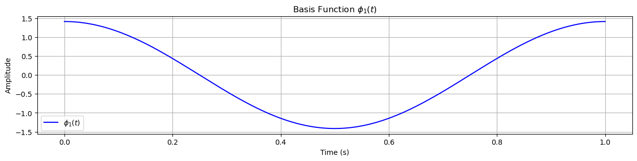
# φ₁(t) = √(2/T) cos(2πt/T) -> In-phase component
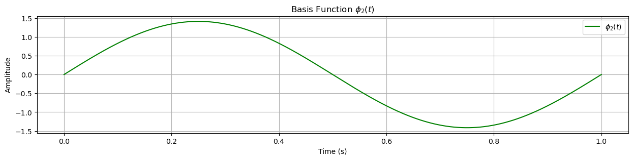
# φ₂(t) = √(2/T) sin(2πt/T) -> Quadrature component
phi1 = np.sqrt(2/T) * np.cos(2 * np.pi * t / T)
phi2 = np.sqrt(2/T) * np.sin(2 * np.pi * t / T)
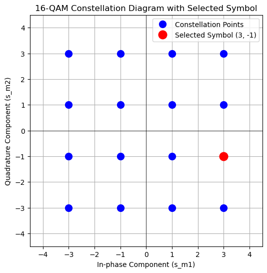
# 2. Generate the 16-QAM constellation points
# Define amplitude levels for 16-QAM (commonly -3, -1, 1, 3)
levels = np.array([-3, -1, 1, 3])
# Create a grid of constellation points (each point is [I, Q])
I, Q = np.meshgrid(levels, levels)
I = I.flatten() # In-phase coordinates (s_m1)
Q = Q.flatten() # Quadrature coordinates (s_m2)
# 3. Select a specific constellation point (symbol)
# For demonstration, we choose the constellation point (s_m1, s_m2) = (3, -1)
s_m1 = 3 # In-phase amplitude
s_m2 = -1 # Quadrature amplitude
# Plot the constellation again, highlighting the selected symbol
plt.figure(figsize=(6,6))
plt.plot(I, Q, 'bo', markersize=10, label='Constellation Points')
plt.plot(s_m1, s_m2, 'ro', markersize=12, label='Selected Symbol (3, -1)')
plt.title('16-QAM Constellation Diagram with Selected Symbol')
plt.xlabel('In-phase Component (s_m1)')
plt.ylabel('Quadrature Component (s_m2)')
plt.grid(True)
plt.axhline(0, color='black', linewidth=0.5)
plt.axvline(0, color='black', linewidth=0.5)
plt.legend()
plt.xlim(-4.5, 4.5)
plt.ylim(-4.5, 4.5)
plt.show()
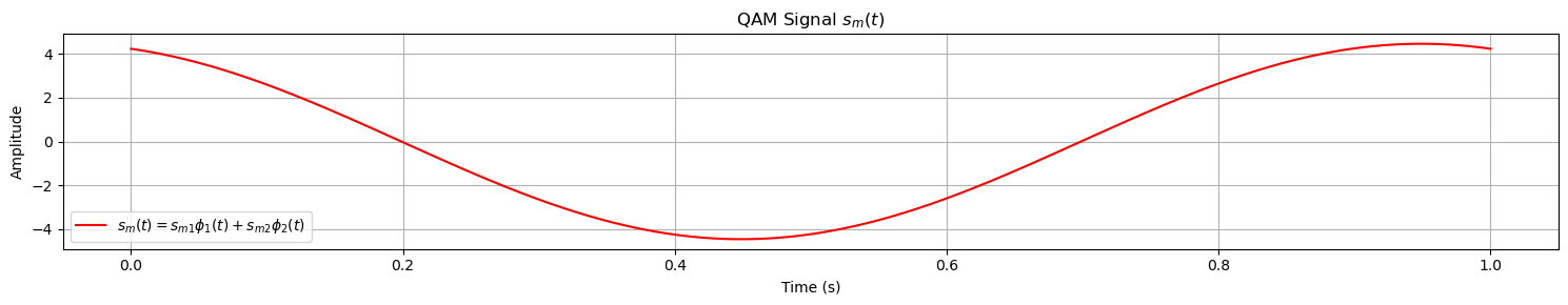
# 4. Generate the time-domain QAM signal s_m(t)
# According to the signal model:
# s_m(t) = s_m1 * φ₁(t) + s_m2 * φ₂(t)
s_m_t = s_m1 * phi1 + s_m2 * phi2
# Optionally, compute the energy of s_m(t) via numerical integration.
# Because φ₁ and φ₂ are orthonormal, the energy should be s_m1² + s_m2².
energy = np.trapz(s_m_t**2, t)
print(f"Computed Energy of s_m(t): {energy:.2f} (Expected: {s_m1**2 + s_m2**2})")
# 5. Plot the basis functions and the resulting signal s_m(t)
# Plot φ₁(t)
plt.figure(figsize=(15, 3))
plt.plot(t, phi1, 'b-', label=r'$\phi_1(t)$')
plt.title(r'Basis Function $\phi_1(t)$')
plt.xlabel('Time (s)')
plt.ylabel('Amplitude')
plt.grid(True)
plt.legend()
# Plot φ₂(t)
plt.figure(figsize=(15, 3))
plt.plot(t, phi2, 'g-', label=r'$\phi_2(t)$')
plt.title(r'Basis Function $\phi_2(t)$')
plt.xlabel('Time (s)')
plt.ylabel('Amplitude')
plt.grid(True)
plt.legend()
# Plot the QAM signal s_m(t)
plt.figure(figsize=(15, 3))
plt.plot(t, s_m_t, 'r-', label=r'$s_m(t) = s_{m1}\phi_1(t) + s_{m2}\phi_2(t)$')
plt.title(r'QAM Signal $s_m(t)$')
plt.xlabel('Time (s)')
plt.ylabel('Amplitude')
plt.grid(True)
plt.legend()
plt.tight_layout()
plt.show()
Computed Energy of s_m(t): 10.00 (Expected: 10)
Energy of QAM Signals#
The energy \( \mathcal{E}_m \) of the signal \( s_m(t) \) is defined as the squared norm of its vector representation:
Substitute the expressions for \( s_{m1} \) and \( s_{m2} \):
Therefore, the total energy becomes:
Euclidean Distance in QAM#
The Euclidean distance between two signal vectors in a QAM constellation is:
where:
\( A_{mi} \) and \( A_{mq} \): In-phase and quadrature amplitudes of symbol \( m \).
\( A_{ni} \) and \( A_{nq} \): In-phase and quadrature amplitudes of symbol \( n \).
\( \mathcal{E}_g \): Energy of the pulse \( g(t) \).
Special Case: Rectangular Constellation#
In a rectangular QAM constellation, the signal amplitudes take discrete values:
The minimum distance between adjacent constellation points is:
which is the same as for PAM. This indicates that the spacing between neighboring points in the constellation determines noise resilience.
Average Energy in Rectangular QAM#
For a rectangular QAM constellation with \( M = 2^{2k_1} \) (e.g., \( M = 4, 16, 64, 256, \ldots \)) and amplitudes \( \pm 1, \pm 3, \ldots, \pm (\sqrt{M} - 1) \) in both directions:
Substituting and simplifying:
Energy Per Bit in QAM#
The average energy per bit in QAM is:
Minimum Distance in Terms of \( \mathcal{E}_{\text{b,avg}} \)#
Using \( d_{\text{min}} = \sqrt{2\mathcal{E}_g} \) and substituting \( \mathcal{E}_{\text{b,avg}} \), the minimum distance can be expressed as:
Unifying Bandpass PAM, PSK, and QAM Signaling Schemes#
General Form of Bandpass Signaling#
All bandpass signaling schemes (PAM, PSK, and QAM) can be expressed in the general form:
where:
\( g(t) \): Signal pulse that defines the time-domain waveform.
\( f_c \): Carrier frequency.
\( A_m \): A parameter determined by the specific signaling scheme.
Definition of \( A_m \) for Different Schemes#
The parameter \( A_m \) distinguishes the signaling schemes:
PAM (Pulse Amplitude Modulation):
\( A_m \) is real and typically takes values:
\[ A_m = \pm1, \pm3, \ldots, \pm(M - 1) \]
PSK (\( M \)-ary Phase Shift Keying):
\( A_m \) is complex and represents a phase shift:
\[ A_m = e^{j \frac{2\pi}{M} (m-1)} \]
QAM (Quadrature Amplitude Modulation):
\( A_m \) is a general complex number, representing both amplitude and phase:
\[ A_m = A_{mi} + jA_{mq} \]where \( A_{mi} \) and \( A_{mq} \) are the in-phase and quadrature components, respectively.
Relationship Between PAM, PSK, and QAM#
Unified Family:
PAM, PSK, and QAM belong to the same family of modulation schemes because they share the same general mathematical structure.
PAM and PSK can be seen as special cases of QAM:
PAM only uses amplitude variations (\( A_m \) is real).
PSK only uses phase variations (\( A_m \) is purely rotational).
Information Carrying Mechanism:
PAM: Only the amplitude of \( A_m \) carries information.
PSK: Only the phase of \( A_m \) carries information.
QAM: Both amplitude and phase of \( A_m \) carry information.
Dimensionality of the Signal Space#
The dimensionality of the signal space for these schemes is determined by the number of orthogonal components required to represent the signal:
PAM: \( N = 1 \) (one-dimensional).
PSK and QAM: \( N = 2 \) (two-dimensional, using orthogonal basis functions for the in-phase and quadrature components).
Importantly, the signal space dimensionality is independent of the constellation size \( M \). For example:
\( M = 4 \) (QPSK) and \( M = 16 \) (16-QAM) both use a two-dimensional signal space.
A table comparing PAM, PSK, and QAM:
Signaling Scheme |
Signal Expression \( s_m(t) \) |
Vector Representation \( s_m \) |
Average Energy \( \mathcal{E}_{\text{avg}} \) |
Energy per Bit \( \mathcal{E}_{\text{b,avg}} \) |
Minimum Distance \( d_{\text{min}} \) |
|---|---|---|---|---|---|
PAM using \(p(t)\) |
\( A_m p(t) \) |
\( A_m \sqrt{\mathcal{E}_p} \) |
\( \frac{2(M^2 - 1)}{3} \mathcal{E}_p \) |
\( \frac{2(M^2 - 1)}{3 \log_2 M} \mathcal{E}_p \) |
\( 2 \sqrt{\mathcal{E}_p} \) |
PAM using \(g(t)\) |
\( A_m g(t) \cos(2\pi f_c t) \) |
\( A_m \sqrt{\frac{\mathcal{E}_g}{2}} \) |
\( \frac{M^2 - 1}{3} \mathcal{E}_g \) |
\( \frac{M^2 - 1}{3 \log_2 M} \mathcal{E}_g \) |
\( \sqrt{2 \mathcal{E}_g} \) |
PSK |
\( g(t) \cos \left[ 2\pi f_c t + \frac{2\pi}{M} (m - 1) \right] \) |
\( \sqrt{\frac{\mathcal{E}_g}{2}} \left[ \cos \frac{2\pi(m-1)}{M}, \sin \frac{2\pi(m-1)}{M} \right] \) |
\( \mathcal{E}_g \) |
\( \frac{\mathcal{E}_g}{\log_2 M} \) |
\( 2 \sqrt{\log_2 M \sin^2 \frac{\pi}{M} \mathcal{E}_{\text{b,avg}}} \) |
QAM |
\( A_{mi} g(t) \cos(2\pi f_c t) - A_{mq} g(t) \sin(2\pi f_c t) \) |
\( \sqrt{\frac{\mathcal{E}_g}{2}} \left[ A_{mi}, A_{mq} \right] \) |
\( \frac{M - 1}{3} \mathcal{E}_g \) |
\( \frac{(M - 1)}{3 \log_2 M} \mathcal{E}_g \) |
\( \sqrt{\frac{6 \log_2 M}{M - 1} \mathcal{E}_{\text{b,avg}}} \) |
Explanation of Columns:
Signal Expression \( s_m(t) \): The time-domain representation of the transmitted signal.
Vector Representation \( s_m \): The signal’s representation in signal space, with dimensionality dependent on the scheme.
Average Energy \( \mathcal{E}_{\text{avg}} \): Average energy per symbol.
Energy per Bit \( \mathcal{E}_{\text{b,avg}} \): Derived by dividing \( \mathcal{E}_{\text{avg}} \) by the number of bits per symbol (\( \log_2 M \)).
Minimum Distance \( d_{\text{min}} \): The minimum Euclidean distance between constellation points, which determines noise resilience.