Example: Band-Limited White Gaussian Noise Process#
In this example, assume that the autocorrelation of a zero-mean, real Gaussian process \( X(t) \) is given by
Let \( V(t) = X^2(t) \).
The autocorrelation and power spectral density of the process \( V(t) = X^2(t) \) are determined in this example.
The autocorrelation function of \( V(t) \) is given by
The corresponding power spectral density is
where
and
Process \(X(t)\)#
We will start by interpreting the provided autocorrelation function and the power spectral density.
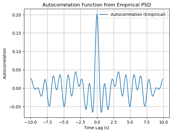
Autocorrelation Function#
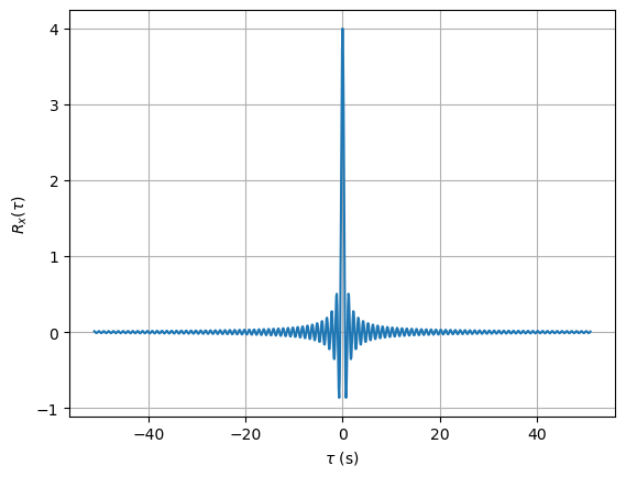
The autocorrelation function \( R_{X}(\tau) \) is given by:
This function is commonly known as the sinc function, which is a characteristic of a band-limited process.
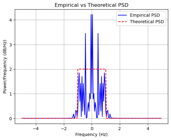
Power Spectral Density (PSD)#
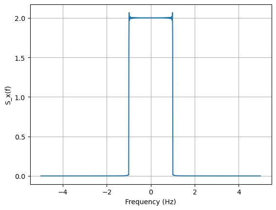
The power spectral density \( S_{X}(f) \) is provided as:
This PSD indicates that the process \( x(t) \) is band-limited to \( B/2 \) Hz, and it has a flat spectrum within this band.
Interpreting the Process \( X(t) \)#
Given that \( X(t) \) is a zero-mean, real Gaussian process with the specified autocorrelation and PSD, we can conclude that \( X(t) \) is a band-limited white Gaussian noise process. The sinc autocorrelation function suggests a band-limited process, and the flat PSD indicates that within the band \( |f| < B/2 \), the power is constant.
import numpy as np
from scipy.signal import butter, lfilter
from scipy.signal.windows import hamming
import matplotlib.pyplot as plt
import warnings
warnings.filterwarnings("ignore")

# Parameters
B = 2  # Bandwidth in Hz
N0 = 1  # Power spectral density level
Fs = 10  # Sampling frequency in Hz
T = 20  # Duration of the signal in seconds
N = int(T * Fs)  # Number of samples

# Time vector
t = np.arange(N) / Fs

# Generate white Gaussian noise
x = np.sqrt(N0 * Fs) * np.random.randn(N)

# Design a low-pass filter to band-limit the noise
f_cutoff = B / 2  # Cutoff frequency
b, a = butter(6, f_cutoff / (Fs / 2))  # 6th order Butterworth filter

# Apply the filter to the noise
x_bandlimited = lfilter(b, a, x)

# Compute the empirical PSD using FFT
X = np.fft.fft(x_bandlimited, n=N)
PSD_empirical = (1 / (Fs * N)) * np.abs(X) ** 2
PSD_empirical = np.fft.fftshift(PSD_empirical)  # Shift zero frequency component to the center
f = np.fft.fftshift(np.fft.fftfreq(N, d=1/Fs))  # Frequency vector for both positive and negative frequencies

# Theoretical PSD
PSD_theoretical = 2 * N0 * (np.abs(f) <= B / 2)

# Plotting
plt.figure()
plt.plot(f, PSD_empirical, 'b', linewidth=1.5, label='Empirical PSD')
plt.plot(f, PSD_theoretical, 'r--', linewidth=1.5, label='Theoretical PSD')
plt.xlabel('Frequency (Hz)')
plt.ylabel('Power/Frequency (dB/Hz)')
plt.title('Empirical vs Theoretical PSD')
plt.legend()
plt.grid(True)
plt.show()
import numpy as np
from scipy.signal import butter, lfilter
from scipy.signal.windows import hamming
import matplotlib.pyplot as plt
import warnings
warnings.filterwarnings("ignore")
# Parameters
B = 2 # Bandwidth in Hz
N0 = 1 # Power spectral density level
Fs = 10 # Sampling frequency in Hz
T = 20 # Duration of the signal in seconds
N = int(T * Fs) # Number of samples
# Time vector
t = np.arange(N) / Fs
# Generate white Gaussian noise
x = np.sqrt(N0 * Fs) * np.random.randn(N)
# Design a low-pass filter to band-limit the noise
f_cutoff = B / 2 # Cutoff frequency
b, a = butter(6, f_cutoff / (Fs / 2)) # 6th order Butterworth filter
# Apply the filter to the noise
x_bandlimited = lfilter(b, a, x)
# Compute the empirical PSD using FFT
# New method to compute the PSD based on Schonhoff's method, Fig. 2.8
X = np.fft.fft(x_bandlimited, n=N)
PSD_empirical = (1 / (Fs * N)) * np.abs(X) ** 2
PSD_empirical = np.fft.fftshift(PSD_empirical) # Shift zero frequency component to the center
f = np.fft.fftshift(np.fft.fftfreq(N, d=1/Fs)) # Frequency vector for both positive and negative frequencies
# Theoretical PSD
PSD_theoretical = 2 * N0 * (np.abs(f) <= B / 2)
# Inverse Fourier Transform to get the autocorrelation function
autocorr_empirical = np.fft.ifftshift(np.fft.ifft(np.fft.ifftshift(PSD_empirical)))
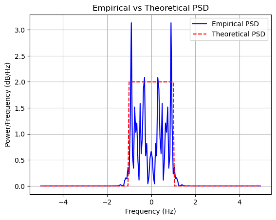
# Plotting the Empirical PSD vs Theoretical PSD
plt.figure()
plt.plot(f, PSD_empirical, 'b', linewidth=1.5, label='Empirical PSD')
plt.plot(f, PSD_theoretical, 'r--', linewidth=1.5, label='Theoretical PSD')
plt.xlabel('Frequency (Hz)')
plt.ylabel('Power/Frequency (dB/Hz)')
plt.title('Empirical vs Theoretical PSD')
plt.legend()
plt.grid(True)
plt.show()
# Plotting the Autocorrelation Function
plt.figure()
plt.plot(t - T/2, np.real(autocorr_empirical), linewidth=1.5, label='Autocorrelation (Empirical)')
plt.xlabel('Time Lag (s)')
plt.ylabel('Autocorrelation')
plt.title('Autocorrelation Function from Empirical PSD')
plt.legend()
plt.grid(True)
plt.show()
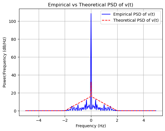
Process \(V(t)\)#
To simulate the process \(V(t) = X^2(t)\), compute its empirical PSD, and plot the theoretical PSD, we will proceed with the following steps in Python:
Generate \(X(t)\) as a band-limited Gaussian noise process.
Generate \(V(t)\) as the square of \(X(t)\).
Compute the empirical PSD of \(V(t)\).
Calculate the theoretical PSD of \(V(t)\) and plot it for comparison.
import numpy as np
from scipy.signal import butter, lfilter
import matplotlib.pyplot as plt

# Parameters
B = 2  # Bandwidth in Hz
N0 = 1  # Power spectral density level
Fs = 10  # Sampling frequency in Hz
T = 20  # Duration of the signal in seconds
N = int(T * Fs)  # Number of samples

# Time vector
t = np.arange(N) / Fs

# Generate white Gaussian noise
x = np.sqrt(N0 * Fs) * np.random.randn(N)

# Design a low-pass filter to band-limit the noise
f_cutoff = B / 2  # Cutoff frequency
b, a = butter(6, f_cutoff / (Fs / 2))  # 6th order Butterworth filter

# Apply the filter to the noise
x_bandlimited = lfilter(b, a, x)

# Generate v(t) = x^2(t)
v = x_bandlimited**2

# Compute the empirical PSD of v(t) using FFT
V = np.fft.fft(v, n=N)
PSD_empirical_v = (1 / (Fs * N)) * np.abs(V) ** 2
PSD_empirical_v = np.fft.fftshift(PSD_empirical_v)  # Shift zero frequency component to the center
f = np.fft.fftshift(np.fft.fftfreq(N, d=1/Fs))  # Frequency vector for both positive and negative frequencies

# Theoretical PSD of v(t)
# C(f) calculation
def theoretical_psd_x(f):
    return 2 * N0 * (np.abs(f) < B / 2)

def C(f):
    f_range = np.linspace(-Fs/2, Fs/2, N)
    S_x_f = theoretical_psd_x(f_range)
    S_x_f_shifted = theoretical_psd_x(f[:, None] - f_range)
    return np.trapz(S_x_f * S_x_f_shifted, f_range, axis=-1)


S_v_f = (2 * N0 * B) ** 2 * (f == 0) + 2 * C(f)

# Plotting
plt.figure()
plt.plot(f, PSD_empirical_v, 'b', linewidth=1.5, label='Empirical PSD of v(t)')
plt.plot(f, S_v_f, 'r--', linewidth=1.5, label='Theoretical PSD of v(t)')
plt.xlabel('Frequency (Hz)')
plt.ylabel('Power/Frequency (dB/Hz)')
plt.title('Empirical vs Theoretical PSD of v(t)')
plt.legend()
plt.grid(True)
plt.show()
Schonhoff’s Simulation#
import numpy as np
import matplotlib.pyplot as plt
def cnv(b, n):
f0 = b / 2 # Center frequency
ts = 0.1 # Sampling interval
ts2 = ts / 2
fi = 1 / ts # Nyquist frequency
df = 1 / (n * ts) # Frequency resolution
n2 = n // 2
ni2 = n2 * ts
# Time vector centered around zero
t = np.arange(-ni2, ni2, ts)
# Autocorrelation function
r = 4 * np.sinc(2 * t)
# Fourier Transform of the autocorrelation function
h = ts * np.fft.fftshift(np.fft.fft(r, n))
mh = np.abs(h)
# Frequency vector for plotting Sx(f)
f = np.arange(-n2, n2) * df
# Power spectral density Sx(f)
plt.figure()
plt.plot(f, mh)
plt.xlabel('Frequency (Hz)')
plt.ylabel('S_x(f)')
plt.grid(True)
plt.show()
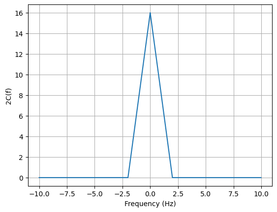
# Convolution to obtain 2C(f)
fc = 2 * np.convolve(h, h) / (n * ts)
# Frequency vector for plotting 2C(f)
fl = np.arange(-len(fc)//2, len(fc)//2) * df
# Power spectral density 2C(f)
plt.figure()
plt.plot(fl, np.abs(fc))
plt.xlabel('Frequency (Hz)')
plt.ylabel('2C(f)')
plt.grid(True)
plt.show()
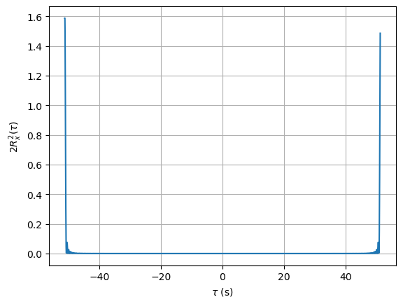
# Inverse Fourier Transform to obtain autocorrelation of squared process
g = np.fft.ifftshift(np.fft.ifft(fc))
# Time vector for plotting 2Rx(tau)^2
tt = np.arange(-n + 1, n) * ts2
# Autocorrelation Rx(tau)
plt.figure()
plt.plot(t, r)
plt.xlabel(r'$\tau$ (s)')
plt.ylabel(r'$R_x(\tau)$')
plt.grid(True)
plt.show()
# Autocorrelation 2Rx(tau)^2
plt.figure()
plt.plot(tt, np.abs(g))
plt.xlabel(r'$\tau$ (s)')
plt.ylabel(r'$2R_x^2(\tau)$')
plt.grid(True)
plt.show()
return fc
# Example usage:
b = 100 # Bandwidth in Hz
n = 1024 # Number of samples
fc = cnv(b, n)