Equivalent Baseband Noise Model#
Baseband Noise Model in Passband Communication Systems
In communication systems, accurately modeling noise is essential for designing robust and efficient transmission schemes.
The Baseband Noise Model offers a framework to analyze how noise affects both passband and baseband signals.
This model facilitates the translation of noise characteristics from the passband to the baseband, enabling simpler and more effective signal processing.
Discussion: Noise Originates at Passband
Note that noise is inherently a passband phenomenon as it affects the transmitted passband signal during its journey through the channel.
Upon reception, this passband noise is converted to baseband noise through downconversion processes, allowing for more straightforward analysis and processing in the baseband domain.
From passband noise to baseband noise process#
Passband Noise \( n(t) \): At the receiver, the received signal typically includes passband noise \( n(t) \).
This noise exists in the passband centered around the carrier frequency \( f_c \) and is typically modeled as additive Gaussian noise.
In-phase \( I(t) \) and Quadrature \( Q(t) \) Components: To convert the passband noise \( n(t) \) to its baseband equivalent, we separate it into two components:
\( I(t) \): The in-phase component, obtained by multiplying \( n(t) \) by \( \cos(2\pi f_c t) \) and passing it through a low-pass filter (LPF).
\( Q(t) \): The quadrature component, obtained by multiplying \( n(t) \) by \( \sin(2\pi f_c t) \) and passing it through a low-pass filter (LPF).
Mathematically, we can express the passband noise \( n(t) \) as:
\[ n(t) = I(t)\cos(2\pi f_c t) - Q(t)\sin(2\pi f_c t) \]Forming Baseband Noise \( n_b(t) \): Once we have \( I(t) \) and \( Q(t) \), we can combine them into a complex baseband noise \( n_b(t) \), which represents the noise in the baseband.
This complex baseband noise is:
\[ n_b(t) = I(t) + jQ(t) \]This is the equivalent baseband representation of the passband noise.
The real part \( I(t) \) represents the in-phase noise, and the imaginary part \( Q(t) \) represents the quadrature noise.
This is sometimes called the “analytic signal” in baseband.
Relationship Between \( n(t) \) and \( n_b(t) \): The original passband noise \( n(t) \) can be related to the baseband noise \( n_b(t) \) through the following expression:
\[ n(t) = \Re\{n_b(t) e^{j2\pi f_c t}\} \]This shows that the passband noise is the real part of the complex baseband noise \( n_b(t) \) modulated up to the carrier frequency \( f_c \).
Summary of the Process:
The passband noise \( n(t) \) exists first in the receiver at the passband.
We separate \( n(t) \) into its in-phase \( I(t) \) and quadrature \( Q(t) \) components.
Using \( I(t) \) and \( Q(t) \), we form the complex baseband noise \( n_b(t) = I(t) + jQ(t) \), which is the baseband equivalent of the passband noise.
Overview of Noise in Communication Systems#
Passband Noise \( n(t) \)#
Definition: \( n(t) \) represents the noise present in the passband channel.
Noise in communication systems typically arises from various sources like thermal agitation, interference, and other environmental factors.
Characteristics:
Wide-Sense Stationary (WSS): The noise \( n(t) \) is modeled as a Wide-Sense Stationary (WSS) process, meaning its statistical properties, such as mean and autocorrelation, are invariant over time.
Real-Valued: Since \( n(t) \) operates in the passband, it is a real-valued signal.
Baseband Noise \( n_b(t) \)#
Definition: \( n_b(t) \) is the equivalent baseband noise obtained by demodulating the passband noise \( n(t) \).
Representation:
\[ \boxed{ n_b(t) = I(t) + jQ(t) } \]where:
\( I(t) \): In-phase component of the baseband noise.
\( Q(t) \): Quadrature component of the baseband noise.
Characteristics:
Complex-Valued: \( n_b(t) \) is a complex-valued signal, capturing both amplitude and phase variations of the noise.
WSS: Similar to \( n(t) \), \( n_b(t) \) is modeled as a WSS process.
Note that the notation \( z \) and \( n_b \) are interchangeably used to represent baseband noise.
Noisy Passband Channel Model#
The noisy passband channel model describes how the transmitted signal \( x(t) \) is affected by the channel impulse response \( h(t) \) and noise \( n(t) \). The model is expressed as:
where
\( y(t) \): Received passband signal.
\( h(t) \): Passband channel impulse response.
\( x(t) \): Transmitted passband signal.
\(*\): Convolution operation.
\( n(t) \): Additive noise in the passband channel.
Detail operations:
Convolution \( h(t) * x(t) \): Represents the effect of the channel on the transmitted signal, including attenuation, delay, and distortion.
Additive Noise \( n(t) \): Represents the noise introduced by the channel during transmission.
Equivalent Baseband Noise Model#
The passband noisy channel is transformed into its equivalent baseband model:
where
\( y_b(t) \): Received baseband signal.
\( h_b(t) \): Equivalent baseband channel response (complex-valued).
\( x_b(t) \): Transmitted baseband signal (complex-valued).
\( n_b(t) \): Baseband noise (complex-valued, WSS).
\(*\): Convolution operation.
Noise Transformation#
Since \( n(t) \) operates in the passband, it must be real-valued.
Therefore, we have
Detail Operations
\( n_b(t) e^{j2\pi f_c t} \): Modulates the baseband noise \( n_b(t) \) up to the carrier frequency \( f_c \).
\( \Re\{ \cdot \} \): Extracts the real part of the complex signal, ensuring \( n(t) \) remains real-valued.
\( \sqrt{2} \): Scaling factor to maintain power consistency between passband and baseband representations.
Deriving \( I(t) \) and \( Q(t) \) from Passband Noise \( n(t) \)#
In a communication system where noise exists in the passband, the In-phase (\( I(t) \)) and Quadrature (\( Q(t) \)) components of the baseband noise \( n_b(t) = I(t) + jQ(t) \) are derived from the passband noise \( n(t) \).
To express \( I(t) \) and \( Q(t) \) in terms of the passband noise \( n(t) \), we perform downconversion (also known as demodulation).
This process involves mixing the passband noise with the carrier signal and then applying a low-pass filter to isolate the desired components.
Mathematical Steps#
Passband to Baseband Conversion:
The passband noise \( n(t) \) is related to the baseband noise \( n_b(t) \) through the following equation:
\[ n(t) = \sqrt{2} \cdot \Re\{ n_b(t) e^{j2\pi f_c t} \} \]Expanding \( n_b(t) \):
\[ n(t) = \sqrt{2} \cdot \Re\{ [I(t) + jQ(t)] e^{j2\pi f_c t} \} \]\[ n(t) = \sqrt{2} \left[ I(t) \cos(2\pi f_c t) - Q(t) \sin(2\pi f_c t) \right] \]Extracting \( I(t) \) and \( Q(t) \):
To isolate \( I(t) \) and \( Q(t) \), perform the following steps:
Multiplication with Carrier Signals:
Multiply \( n(t) \) by \( \sqrt{2} \cos(2\pi f_c t) \) and \( \sqrt{2} \sin(2\pi f_c t) \) to extract \( I(t) \) and \( Q(t) \), respectively.
\[ n(t) \cdot \sqrt{2} \cos(2\pi f_c t) = 2 \left[ I(t) \cos^2(2\pi f_c t) - Q(t) \sin(2\pi f_c t) \cos(2\pi f_c t) \right] \]\[ n(t) \cdot \sqrt{2} \sin(2\pi f_c t) = 2 \left[ I(t) \sin(2\pi f_c t) \cos(2\pi f_c t) - Q(t) \sin^2(2\pi f_c t) \right] \]Applying Low-Pass Filtering (LPF):
The high-frequency components (oscillating at \( 2f_c \)) are removed by the LPF, leaving only the baseband components.
\[ \text{LPF} \left\{ n(t) \cdot \sqrt{2} \cos(2\pi f_c t) \right\} = I(t) \]\[ \text{LPF} \left\{ -n(t) \cdot \sqrt{2} \sin(2\pi f_c t) \right\} = Q(t) \]Note: The negative sign in the \( Q(t) \) extraction accounts for the phase shift introduced during multiplication.
Final Expressions for \( I(t) \) and \( Q(t) \):
Combining the above steps, the mathematical expressions for \( I(t) \) and \( Q(t) \) in terms of the passband noise \( n(t) \) are:
\[ I(t) = \text{LPF} \left\{ \sqrt{2} \cdot n(t) \cdot \cos(2\pi f_c t) \right\} \]\[ Q(t) = \text{LPF} \left\{ -\sqrt{2} \cdot n(t) \cdot \sin(2\pi f_c t) \right\} \]Alternatively, removing the negative sign by redefining the quadrature component:
\[ Q(t) = \text{LPF} \left\{ \sqrt{2} \cdot n(t) \cdot \sin(2\pi f_c t) \right\} \](The negative sign can be absorbed into the definition of \( Q(t) \), depending on the system’s phase conventions.)
Finally, we have
Autocorrelation Function (ACF)#
In communication systems, accurately characterizing noise is essential.
Understanding the Autocorrelation Function (ACF) and Power Spectral Density (PSD) of both bandpass noise and its baseband equivalent provides critical insights into how noise impacts signal integrity and system performance.
The Autocorrelation Function (ACF) measures the similarity between a signal and a delayed version of itself as a function of the delay.
Baseband Noise \( n_b(t) \) ACF#
Given:
Autocorrelation Function:
Assumptions:
Zero Mean: \( \mathbb{E}\{ I(t) \} = \mathbb{E}\{ Q(t) \} = 0 \)
Independence: \( \mathbb{E}\{ I(t)Q(t + \tau) \} = 0 \)
Identical Statistics: \( \mathbb{E}\{ I(t)I(t + \tau) \} = \mathbb{E}\{ Q(t)Q(t + \tau) \} = R_I(\tau) \)
Simplification:
Final ACF for baseband noise:
Passband Noise \( n(t) \) ACF#
Given:
Autocorrelation Function:
Expanding the product:
Applying assumptions:
Zero Mean: Cross terms involving \( I(t)Q(t + \tau) \) vanish.
Identical Statistics: \( \mathbb{E}\{ I(t)I(t + \tau) \} = \mathbb{E}\{ Q(t)Q(t + \tau) \} = R_I(\tau) \)
Simplified expression:
Final ACF for passband noise:
Express \( R_n(\tau) \) as the Real Part of \( R_{n_b}(\tau) \) Modulated by the Carrier
We have
and
So
Finally
Power Spectral Density (PSD) of Noise#
The Power Spectral Density (PSD) represents how the power of a signal or noise process is distributed across different frequency components.
It is the Fourier Transform of the Autocorrelation Function.
Baseband Noise \( n_b(t) \) PSD#
Given:
PSD definition:
where:
\( S_I(f) \): PSD of the in-phase noise component \( I(t) \).
Final PSD for daseband noise:
Passband Noise \( n(t) \) PSD#
Given:
PSD definition:
Using Fourier Transform property:
Substituting back:
Final PSD for passband noise:
Other Relationships#
The relationship between the baseband noise PSD \( S_{n_b}(f) \) and the passband noise PSD \( S_n(f) \) is:
There’s no need to cut off the PSD at \( f+f_c \leq 0 \) since the passband noise contains symmetric components about the carrier frequency.
The relationship should reflect the fact that the baseband noise spectrum is derived from the shifted passband spectrum, and it exists only in the positive frequency range.
The relationship between the passband noise PSD \( S_n(f) \) and the baseband noise PSD \( S_{n_b}(f) \) is:
This expression captures the fact that the passband noise PSD is composed of the baseband noise PSD shifted by the carrier frequency \( f_c \) in both positive and negative frequency directions.
White Noise Spectral Density \( N_0 / 2 \)#
Given the passband noise PSD \( S_n(f) \) for white noise with spectral density \( \frac{N_0}{2} \) in the passband as:
We have the relationship between the passband PSD \( S_n(f) \) and the baseband PSD \( S_{n_b}(f) \) is:
To find the baseband PSD \( S_{n_b}(f) \), we need to shift the passband PSD down by \( f_c \) and combine the components:
For \( f \in \left[ -\frac{W}{2}, \frac{W}{2} \right] \):
The baseband PSD \( S_{n_b}(f) \) corresponds to the passband PSD \( S_n(f + f_c) \), shifted back to baseband.
From the passband PSD \( S_n(f) = \frac{N_0}{2} \), the baseband noise PSD \( S_{n_b}(f) \) within the range \( |f| \leq \frac{W}{2} \) is:
\[ S_{n_b}(f) = 2 \cdot \frac{N_0}{2} = N_0 \]This factor of 2 comes from combining the contributions of both sidebands (upper and lower).
For \( |f| > \frac{W}{2} \):
Outside the baseband range, the passband noise PSD \( S_n(f) = 0 \), so the baseband PSD will also be 0 for \( |f| > \frac{W}{2} \).
Thus, the baseband noise PSD \( S_{n_b}(f) \) is:
Example: PSD of LTI System#
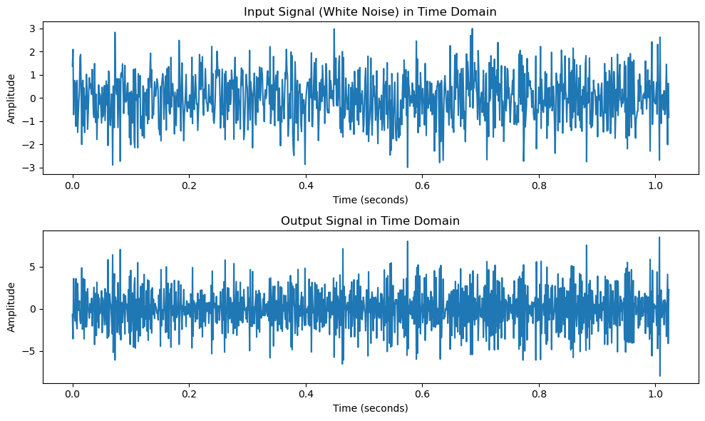
This example demonstrates the analysis of a linear time-invariant (LTI) system excited by white noise, focusing on the input-output relationship in both the time domain and the frequency domain using the Power Spectral Density (PSD).
This example shows how a white noise input is transformed by a system and how its power spectral density is modified based on the system’s frequency response.
Input Signal (White Noise)#
The input to the system is white noise, which is a stochastic process with a constant power spectral density over all frequencies.
The white noise \( x(n) \) is generated with a zero mean and a variance \( \sigma_x^2 \):
\[ x(n) \sim \mathcal{N}(0, \sigma_x^2) \]where \( \sigma_x^2 = 1 \) in this case.
Impulse Response of the System#
The system is described by a simple finite impulse response (FIR) filter with an impulse response \( h(n) \):
This is a second-order difference equation, which can represent a simple smoothing or filtering operation.
Output Signal (Convolution)#
The output of the system is the result of convolving the input signal \( x(n) \) with the system’s impulse response \( h(n) \):
Mathematically, convolution is expressed as:
This operation represents how the input signal \( x(n) \) is transformed by the system defined by \( h(n) \).
Power Spectral Density (PSD)#
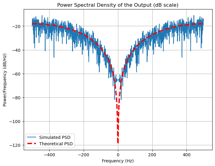
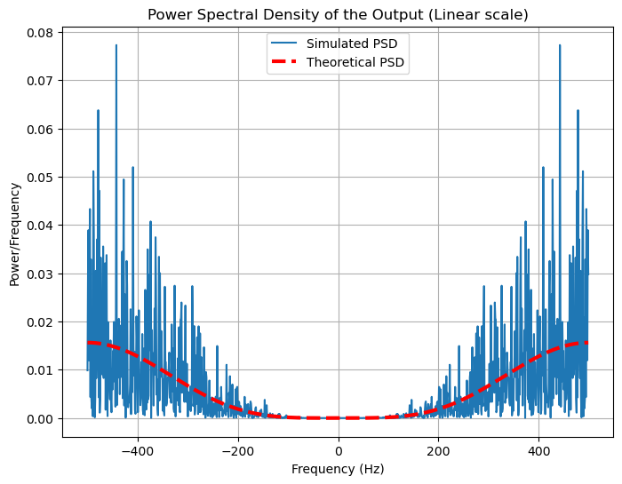
The Power Spectral Density (PSD) describes how the power of a signal is distributed over different frequencies. It can be computed as the magnitude squared of the Fourier transform of the signal, normalized by the signal length and sampling frequency.
The PSD of the input signal \( x(n) \) is:
where \( N \) is the number of samples, and \( f_s \) is the sampling frequency.
Similarly, the PSD of the output signal \( y(n) \) is:
Theoretical Power Spectral Density of the Output#
Since the input is white noise (which has a flat PSD), the output’s PSD is related to the input PSD and the frequency response of the system.
The frequency response of the system can be derived from the Fourier transform of the impulse response \( h(n) \).
The theoretical power spectral density \( S_{yy}(f) \) of the output signal \( y(n) \) is:
where \( H(f) \) is the Fourier transform of the system’s impulse response \( h(n) \), and \( \sigma_x^2 \) is the variance of the white noise input.
For the given impulse response \( h(n) = [1, -2, 1] \), the Fourier transform \( H(f) \) can be computed as:
Simplifying:
Thus, the magnitude squared of the frequency response is:
Therefore, the theoretical PSD of the output is:
where \( f_{\text{normalized}} = \frac{f}{f_s} \) is the frequency normalized by the sampling frequency.
Simulation#
Input: White noise \( x(n) \).
System: FIR filter with impulse response \( h(n) = [1, -2, 1] \).
Output: Convolution of \( x(n) \) with \( h(n) \).
Frequency Domain Analysis: PSD of the output signal is compared with the theoretical PSD derived from the system’s frequency response.
Theoretical Output PSD: \( S_{yy}(f) = 16 \sigma_x^2 \sin^4(\pi f_{\text{normalized}}) \).
import numpy as np
import matplotlib.pyplot as plt
from scipy.fft import fft, fftshift
from scipy.signal import convolve

import warnings
warnings.filterwarnings('ignore')

# Parameters
N = 1024  # Number of points (choose a power of 2 for faster FFT computation)
sigma_x2 = 1  # Variance of the white noise
fs = 1000  # Sampling frequency in Hz

# Generate white noise input
x = np.sqrt(sigma_x2) * np.random.randn(N)

# Impulse response of the system h(n)
h = np.array([1, -2, 1])

# Compute the output signal by convolving the input with the impulse response
y = convolve(x, h, mode='same')

# Compute the frequency vector
f = np.linspace(-fs/2, fs/2, N, endpoint=False)

# Compute the Power Spectral Densities (PSDs)
PSD_x = fftshift(np.abs(fft(x, N))**2) / (N * fs)
PSD_y = fftshift(np.abs(fft(y, N))**2) / (N * fs)

# Theoretical Power Spectral Density
f_normalized = f / fs  # Normalize frequency by the sampling frequency
S_yy_theoretical = 16 * sigma_x2 * np.sin(np.pi * f_normalized)**4

# Time domain plots
plt.figure(figsize=(10, 6))

plt.subplot(2, 1, 1)
plt.plot(np.arange(N) / fs, x)
plt.title('Input Signal (White Noise) in Time Domain')
plt.xlabel('Time (seconds)')
plt.ylabel('Amplitude')

plt.subplot(2, 1, 2)
plt.plot(np.arange(N) / fs, y)
plt.title('Output Signal in Time Domain')
plt.xlabel('Time (seconds)')
plt.ylabel('Amplitude')

plt.tight_layout()
plt.show()

# Frequency domain plot in dB scale
plt.figure(figsize=(8, 6))
plt.plot(f, 10 * np.log10(PSD_y), label="Simulated PSD")
plt.plot(f, 10 * np.log10(S_yy_theoretical / N), 'r--', linewidth=3, label='Theoretical PSD')
plt.title('Power Spectral Density of the Output (dB scale)')
plt.xlabel('Frequency (Hz)')
plt.ylabel('Power/Frequency (dB/Hz)')
plt.legend(loc='best')
plt.grid(True)
plt.show()

# Frequency domain plot in linear scale
plt.figure(figsize=(8, 6))
plt.plot(f, PSD_y, label="Simulated PSD")
plt.plot(f, S_yy_theoretical / N, 'r--', linewidth=3, label='Theoretical PSD')
plt.title('Power Spectral Density of the Output (Linear scale)')
plt.xlabel('Frequency (Hz)')
plt.ylabel('Power/Frequency')
plt.legend(loc='best')
plt.grid(True)
plt.show()


