Orthonormal Expansions#
Complete Orthonormal Expansion#
A set of functions \(\{\Theta_i(t)\}_{i=1}^{\infty}\) is a complete set of orthonormal functions if the following conditions are satisfied:
Orthonormality, which combines orthogonality (zero inner product between distinct functions) and normalization (unit length for each function).
Completeness, which ensures that the orthonormal set forms a complete basis, allowing any function in the space to be expressed as a linear combination of the basis functions.
Orthonormality#
Orthonormality is a fundamental property of a set of functions (or vectors) in a function space (or vector space).
A set of functions \(\{\Theta_i(t)\}\) is said to be orthonormal if each pair of distinct functions is orthogonal, and each function is normalized. Formally, this means:
Orthogonality:
Two functions \(\Theta_i(t)\) and \(\Theta_j(t)\) are orthogonal if their inner product is zero:\[ \langle \Theta_i, \Theta_j \rangle = \int \Theta_i(t) \Theta_j^*(t) \, dt = 0 \quad \text{for } i \neq j. \]Normalization:
Each function is normalized to have unit length:\[ \langle \Theta_i, \Theta_i \rangle = \int |\Theta_i(t)|^2 \, dt = 1. \]
Combining these, the set \(\{\Theta_i(t)\}\) satisfies:
where \(\delta_{ij}\) is the Kronecker delta.
Characterization via the Kronecker Delta Function#
The Kronecker delta function, denoted by \(\delta_{ij}\), serves as a concise way to express the orthonormality condition. It is defined as:
In the context of orthonormal functions, the inner product between any two functions in the set is given by the Kronecker delta:
This equation succinctly captures both orthogonality (when \(i \neq j\)) and normalization (when \(i = j\)) in a single expression.
Completeness#
Completeness ensures that the orthonormal set of functions spans the entire function space under consideration.
This means that any arbitrary function \(s(t)\) within the space can be expressed as a (possibly infinite) linear combination of the orthonormal basis functions:
where the coefficients \(s_i\) are determined by the inner product:
In other words, completeness guarantees that the orthonormal set is sufficient to represent any function in the space without omission.
It ensures that there are no “gaps” in the representation, making the set a complete basis for the function space.
Gram-Schmidt Procedure#
The Gram-Schmidt procedure is a method for constructing an orthonormal set of functions from a given set of linearly independent functions.
Objective#
Given a set of functions \(\{s_i(t)\}_{i=1}^{M}\), the goal is to construct a set of orthonormal functions \(\{\Theta_i(t)\}_{i=1}^{N}\) such that any function \(s_i(t)\) can be expressed as
where the inner product is defined by
Procedure#
Initialize the First Orthonormal Function:
\[ \Theta_1(t) = \frac{s_1(t)}{\sqrt{\langle s_1(t), s_1(t) \rangle}}, \]where
\[ \langle s_i(t), s_j(t) \rangle = \int s_i(t) s_j^*(t) \, dt. \]Orthogonalize and Normalize Subsequent Functions:
For each \(j = 2, \dots, M\), perform the following steps:
a. Orthogonalize:
\[ s_j^{\circ}(t) = s_j(t) - \sum_{i=1}^{j-1} \langle s_j(t), \Theta_i(t) \rangle \Theta_i(t). \]b. Normalize:
\[ \Theta_j(t) = \frac{s_j^{\circ}(t)}{\sqrt{\langle s_j^{\circ}(t), s_j^{\circ}(t) \rangle}}. \]Note: If \(\langle s_j^{\circ}(t), s_j^{\circ}(t) \rangle = 0\), then \(s_j(t)\) is linearly dependent on the previous functions, and \(\Theta_j(t)\) is not added to the orthonormal set.
Finalize the Orthonormal Set:
The process yields a set of non-zero orthonormal functions \(\{\Theta_i(t)\}_{i=1}^{N}\), where \(N \leq M\). These functions form the desired orthonormal basis constructed from the original set \(\{s_i(t)\}_{i=1}^{M}\).
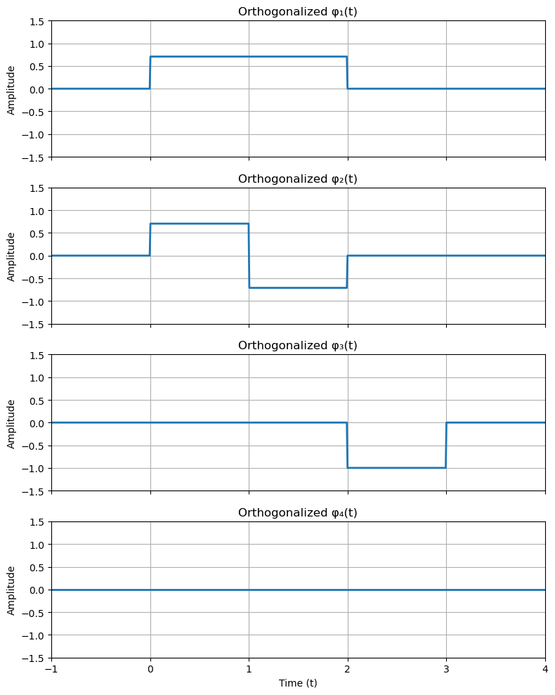
Example: Gram-Schmidt orthogonalization process for rectangular signals#
The Gram-Schmidt process is a method for orthonormalizing a set of vectors (or functions) in an inner product space.
Given a set of linearly independent vectors, the process generates an orthonormal set that spans the same subspace.
Application to Rectangular Signals#
We apply the Gram-Schmidt process to four rectangular signals \( S_1(t), S_2(t), S_3(t), \) and \( S_4(t) \).
\( S_1(t) \): A simple rectangular pulse active from \( t = 0 \) to \( t = 2 \).
\( S_2(t) \): A piecewise signal that is positive from \( t = 0 \) to \( t = 1 \) and negative from \( t = 1 \) to \( t = 2 \).
\( S_3(t) \): A piecewise signal positive from \( t = 0 \) to \( t = 2 \) and negative from \( t = 2 \) to \( t = 3 \).
\( S_4(t) \): A negative rectangular pulse active from \( t = 0 \) to \( t = 3 \).
Orthogonalization Steps and Observations#
Step 1: Orthogonalizing \( S_1(t) \)
Normalization: \( \phi_1(t) = \frac{S_1(t)}{\|S_1(t)\|} \)
Result: A normalized version of \( S_1(t) \).
Step 2: Orthogonalizing \( S_2(t) \) against \( \phi_1(t) \)
Projection: Calculate the component of \( S_2(t) \) along \( \phi_1(t) \).
Orthogonalization: Subtract this projection to obtain \( \phi_2(t) \), ensuring orthogonality to \( \phi_1(t) \).
Normalization: Normalize \( \phi_2(t) \).
Step 3: Orthogonalizing \( S_3(t) \) against \( \phi_1(t) \) and \( \phi_2(t) \)
Projection: Calculate components along both \( \phi_1(t) \) and \( \phi_2(t) \).
Orthogonalization: Subtract these projections to obtain \( \phi_3(t) \), ensuring orthogonality to both \( \phi_1(t) \) and \( \phi_2(t) \).
Normalization: Normalize \( \phi_3(t) \).
Step 4: Orthogonalizing \( S_4(t) \) against \( \phi_1(t) \), \( \phi_2(t) \), and \( \phi_3(t) \)
Projection: Calculate components along \( \phi_1(t) \), \( \phi_2(t) \), and \( \phi_3(t) \).
Orthogonalization: Subtract these projections to obtain \( \phi_4(t) \).
Normalization Check: Compute the energy (squared norm) of \( \phi_4(t) \).
Conclusion
The set of three orthonormal functions \( \{\phi_1, \phi_2, \phi_3\} \) forms a complete orthonormal set for the given set of four signals \( \{S_1, S_2, S_3, S_4\} \).
DISCUSSIONS
Why \( \phi_4(t) \) is Zero: Linear Dependence Explained
Upon orthogonalizing \( S_4(t) \) against the already established orthonormal set \( \{\phi_1(t), \phi_2(t), \phi_3(t)\} \), the resulting \( \phi_4(t) \) was found to be zero (or effectively zero within numerical precision). This outcome is a direct consequence of linear dependence among the signals.
Understanding Linear Dependence:
Definition: A set of vectors (or functions) is linearly dependent if at least one vector (or function) in the set can be expressed as a linear combination of the others.
Implication: If \( S_4(t) \) can be written as a combination of \( S_1(t), S_2(t), \) and \( S_3(t) \), then it does not introduce a new dimension to the space spanned by these functions.
Mathematical Perspective:
Span: The span of \( \{S_1(t), S_2(t), S_3(t)\} \) is the set of all possible linear combinations of these functions.
Membership of \( S_4(t) \): If \( S_4(t) \) lies within this span, it does not extend the space, making it redundant for the purpose of forming a basis.
Result in Gram-Schmidt:
Orthogonalization Outcome: Since \( S_4(t) \) does not introduce a new direction (i.e., it’s within the span of \( \{\phi_1(t), \phi_2(t), \phi_3(t)\} \)), the orthogonalization process yields \( \phi_4(t) = 0 \).
Basis Formation: Only the non-zero orthonormal functions (\( \phi_1(t), \phi_2(t), \phi_3(t) \)) form the final orthonormal basis. \( \phi_4(t) \) is excluded as it doesn’t contribute additional information.
import numpy as np
import warnings
import matplotlib.pyplot as plt
warnings.filterwarnings('ignore')

# Define the time vector with sufficient resolution
t = np.linspace(-2, 5, 1000)  # includes some range before and after the pulses for context

# Define the rectangular pulse signal S1(t)
def S1(t):
    return np.where((t >= 0) & (t <= 2), 1.0, 0.0)

# Define the piecewise signal S2(t)
def S2(t):
    return np.where((t >= 0) & (t < 1), 1.0,
                    np.where((t >= 1) & (t <= 2), -1.0, 0.0))

# Define the piecewise signal S3(t)
def S3(t):
    return np.where((t >= 0) & (t < 2), 1.0,
                    np.where((t >= 2) & (t <= 3), -1.0, 0.0))

# Define the piecewise signal S4(t)
def S4(t):
    return np.where((t >= 0) & (t <= 3), -1.0, 0.0)

# Evaluate the signals
S1_vec = S1(t)
S2_vec = S2(t)
S3_vec = S3(t)
S4_vec = S4(t)

# Plot the original signals
fig, axs = plt.subplots(4, 1, figsize=(8, 10), sharex=True)

# Plot S1(t)
axs[0].plot(t, S1_vec, linewidth=2)
axs[0].set_title('Signal S₁(t)')
axs[0].grid(True)
axs[0].set_ylabel('Amplitude')

# Plot S2(t)
axs[1].plot(t, S2_vec, linewidth=2)
axs[1].set_title('Signal S₂(t)')
axs[1].grid(True)
axs[1].set_ylabel('Amplitude')

# Plot S3(t)
axs[2].plot(t, S3_vec, linewidth=2)
axs[2].set_title('Signal S₃(t)')
axs[2].grid(True)
axs[2].set_ylabel('Amplitude')

# Plot S4(t)
axs[3].plot(t, S4_vec, linewidth=2)
axs[3].set_title('Signal S₄(t)')
axs[3].set_xlabel('Time (t)')
axs[3].grid(True)
axs[3].set_ylabel('Amplitude')

# Set axis limits for all subplots to make the plots clearer
for ax in axs:
    ax.set_xlim([-2, 5])
    ax.set_ylim([-1.5, 1.5])

# Adjust layout and display the figure
plt.tight_layout()
plt.show()
# Gram-Schmidt Process

# Define the inner product using the trapezoidal rule
def inner_product(f, g, t):
    return np.trapz(f * g, t)

# Initialize lists to store orthonormal basis functions
phi = []

# Step 1: Normalize S1
norm_S1 = np.sqrt(inner_product(S1_vec, S1_vec, t))
phi1 = S1_vec / norm_S1
phi.append(phi1)

# Step 2: Make S2 orthogonal to phi1 and normalize
c21 = inner_product(S2_vec, phi1, t)
phi2 = S2_vec - c21 * phi1
norm_phi2 = np.sqrt(inner_product(phi2, phi2, t))
phi2 = phi2 / norm_phi2
phi.append(phi2)

# Step 3: Make S3 orthogonal to phi1 and phi2 and normalize
c31 = inner_product(S3_vec, phi1, t)
c32 = inner_product(S3_vec, phi2, t)
phi3 = S3_vec - c31 * phi1 - c32 * phi2
norm_phi3 = np.sqrt(inner_product(phi3, phi3, t))
phi3 = phi3 / norm_phi3
phi.append(phi3)

# Step 4: Make S4 orthogonal to phi1, phi2, and phi3
c41 = inner_product(S4_vec, phi1, t)
c42 = inner_product(S4_vec, phi2, t)
c43 = inner_product(S4_vec, phi3, t)
phi4 = S4_vec - c41 * phi1 - c42 * phi2 - c43 * phi3
energy_phi4 = inner_product(phi4, phi4, t)

# If phi4 has no energy, it is a linear combination of the previous vectors and can be discarded
threshold = 1e-10  # Threshold for numerical precision
if energy_phi4 < threshold:
    phi4 = np.zeros_like(t)
else:
    phi4 = phi4 / np.sqrt(energy_phi4)
    phi.append(phi4)

# Plot the orthogonalized signals
fig_ortho, axs_ortho = plt.subplots(4, 1, figsize=(8, 10), sharex=True)

# Plot phi1(t)
axs_ortho[0].plot(t, phi[0], linewidth=2)
axs_ortho[0].set_title('Orthogonalized φ₁(t)')
axs_ortho[0].grid(True)
axs_ortho[0].set_ylabel('Amplitude')

# Plot phi2(t)
axs_ortho[1].plot(t, phi[1], linewidth=2)
axs_ortho[1].set_title('Orthogonalized φ₂(t)')
axs_ortho[1].grid(True)
axs_ortho[1].set_ylabel('Amplitude')

# Plot phi3(t)
axs_ortho[2].plot(t, phi[2], linewidth=2)
axs_ortho[2].set_title('Orthogonalized φ₃(t)')
axs_ortho[2].grid(True)
axs_ortho[2].set_ylabel('Amplitude')

# Plot phi4(t)
axs_ortho[3].plot(t, phi4, linewidth=2)
axs_ortho[3].set_title('Orthogonalized φ₄(t)')
axs_ortho[3].set_xlabel('Time (t)')
axs_ortho[3].grid(True)
axs_ortho[3].set_ylabel('Amplitude')

# Set axis limits for all subplots to make the plots clearer
for ax in axs_ortho:
    ax.set_xlim([-1, 4])
    ax.set_ylim([-1.5, 1.5])

# Adjust layout and display the figure
plt.tight_layout()
plt.show()

# Additional Computations and Discussions

# # Compute and print 1/sqrt(2)
# one_over_sqrt2 = 1 / np.sqrt(2)
# print(f"1/sqrt(2) = {one_over_sqrt2}")

# # Compute and print the maximum of phi2
# max_phi2 = np.max(phi2)
# print(f"Maximum value of φ₂(t): {max_phi2}")