Stochastic Process#
A stochastic process, denoted as \(\mathbf{x}(t)\), is a mathematical object that describes a collection of random variables indexed by time or another parameter.
This definition captures how the process evolves over time and how it depends on the outcome of a random experiment \(\zeta\).
Interpretation:#
The interpretation of \(\mathbf{x}(t)\) depends on whether we fix or vary the time \(t\) and the outcome \(\zeta\), leading to different perspectives such as sets of functions, sample paths, random variables, or specific values.
Both \(t\) and \(\zeta\) are Variable:
\(\mathbf{x}(t)\) represents a family or set of functions.
When considering different outcomes \(\zeta\) and different times \(t\), the process gives us different functions \(x(t)\).
Each function corresponds to a different realization of the stochastic process.
\(t\) is Variable, \(\zeta\) is Fixed:
\(\mathbf{x}(t)\) is a non-random function, also called a sample path.
For a fixed outcome \(\zeta = \zeta_0\), the function \(x(t)\) describes how the process behaves over time for that particular outcome.
This function is deterministic once \(\zeta\) is known.
\(t\) is Fixed, \(\zeta\) is Variable:
\(\mathbf{x}(t)\) is a random variable.
At a specific time \(t = t_0\), the value of the process depends on the random experiment \(\zeta\).
Thus, for each fixed \(t_0\), \(\mathbf{x}(t_0)\) is a random variable with a probability distribution that can be studied.
Both \(t\) and \(\zeta\) are Fixed:
\(\mathbf{x}(t)\) takes a specific value.
When both the time and the outcome of the random experiment are fixed, the process \(\mathbf{x}(t)\) reduces to a single value, which is deterministic for that combination of \(t\) and \(\zeta\).
Stationarity#
Strict Stationarity#
Definition: A stochastic process \(\mathbf{x}(t)\) is said to be strictly stationary if its joint probability distribution does not change when shifted in time. In other words, for any set of time points \(t_1, t_2, \dots, t_n\) and for any time shift \(\tau\), the joint distribution of the process at these points is the same as the joint distribution of the process at the shifted points \(t_1 + \tau, t_2 + \tau, \dots, t_n + \tau\).
Mathematical Expression:
Implications:
Invariance: The statistical properties of the process are invariant under time shifts.
Dependence: The process looks the same at any point in time, meaning the distribution functions depend only on the time differences, not on the actual times.
Example: If \(\mathbf{x}(t)\) is a sequence of independent and identically distributed (i.i.d.) random variables, it is strictly stationary because the joint distribution does not change with time shifts.
Strict Cyclo-Stationarity#
Definition: A stochastic process \(\mathbf{x}(t)\) is strictly cyclo-stationary if its joint distribution function is periodic with a fixed period \(T\). This means that the process’s statistical properties repeat every \(T\) units of time.
Mathematical Expression:
Implications:
Periodic Structure: The process exhibits a repeating structure in time.
Applications: This is useful in modeling seasonal data or systems with inherent periodicities, such as daily temperature variations or economic cycles.
Example: Consider a process that models the daily temperature at a specific location, which tends to repeat its pattern every year. This process would be strictly cyclo-stationary with a period of one year.
Wide-Sense Stationarity (WSS)#
Definition: A process \(\mathbf{x}(t)\) is wide-sense stationary (or weakly stationary) if its mean and autocorrelation function do not change with time.
Mathematical Expressions:
Constant Mean:
\[ E\{\mathbf{x}(t)\} = \mu, \quad \forall t \]The mean \(\mu\) is the same for all \(t\).
Time-Invariant Autocorrelation:
\[ R_{\mathbf{x}}(t, t+\tau) = E\{\mathbf{x}(t)\mathbf{x}(t+\tau)\} = R_{\mathbf{x}}(\tau), \quad \forall t, \forall \tau \]The autocorrelation \(R_{\mathbf{x}}(\tau)\) depends only on the time difference \(\tau\), not on the specific times \(t\) and \(t + \tau\).
Implications:
Simplified Analysis: WSS simplifies the analysis and modeling of processes since we only need to consider the time differences.
Common in Applications: Many practical processes (e.g., signal processing) assume WSS due to its manageable properties.
Example: A white noise process with zero mean and constant variance is WSS because its mean and autocorrelation do not vary with time.
Wide-Sense Cyclo-Stationarity#
Definition: A process \(\mathbf{x}(t)\) is wide-sense cyclo-stationary if its mean and autocorrelation function are periodic with a period \(T\).
Mathematical Expressions:
Periodic Mean:
\[ E\{\mathbf{x}(t)\} = E\{\mathbf{x}(t+kT)\}, \quad \forall t, \text{for integer } k \]The mean is periodic with period \(T\).
Periodic Autocorrelation:
\[ R_{\mathbf{x}}(t_1, t_2) = R_{\mathbf{x}}(t_1+kT, t_2+kT), \quad \forall t_1, t_2, \text{for integer } k \]The autocorrelation is also periodic with period \(T\).
Implications:
Periodic Properties: The process exhibits periodic behavior in its second-order statistics (mean and autocorrelation).
Applications: Useful in modeling phenomena with inherent periodicity but where strict cyclo-stationarity might be too strong a requirement.
Transformation to WSS: If \(\mathbf{x}(t)\) is wide-sense cyclo-stationary, then the process \(\mathbf{x}(t+\theta)\), where \(\theta \sim U(0, T)\), is wide-sense stationary. This means that randomly shifting the process within one period transforms it into a WSS process.
Example: Consider an electrical signal with a periodic component superimposed on a stationary noise process. The overall process is wide-sense cyclo-stationary, but shifting it within one period results in a WSS process.
Example: Random Square Wave#
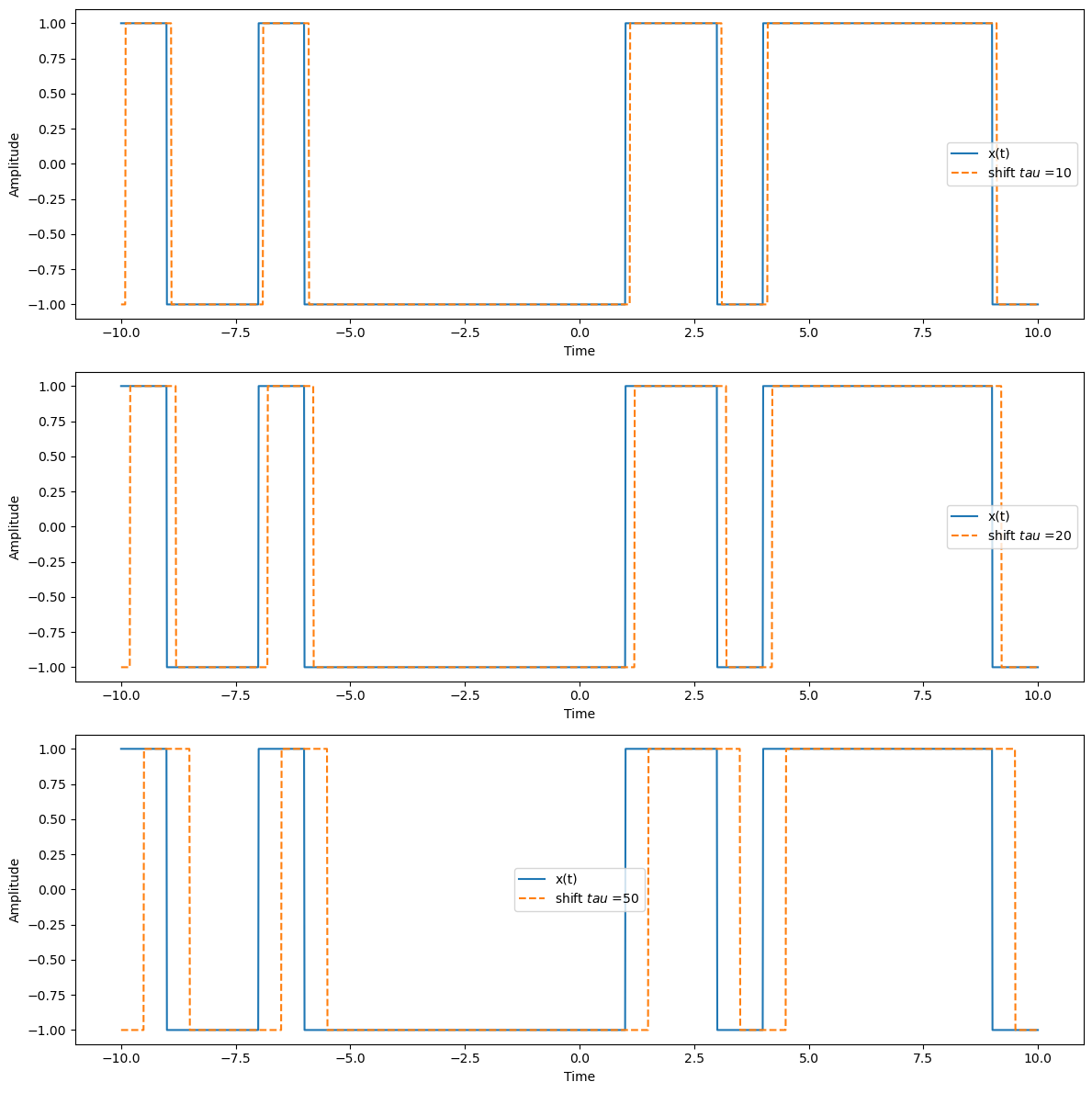
In this example, we consider a stationary and ergodic random process \(\mathbf{x}(t)\) defined by the waveform shown below. The key characteristics of this process are:
The process \(\mathbf{x}(t)\) is real.
During each time interval \(T_c\), the process takes a value of \(+1\) with probability \(\frac{1}{2}\) and \(-1\) with probability \(\frac{1}{2}\).
import numpy as np
import matplotlib.pyplot as plt
import warnings
warnings.filterwarnings("ignore")

# Parameters
T_c = 100       # Duration of each interval
T = 10       # Total duration (from -T to +T)
num_intervals = 2 * T  # Number of intervals (since we go from -T to +T)
t = np.linspace(-T, T, num_intervals * T_c)  # Time vector

# Generate the random process x(t)
np.random.seed(0)  # For reproducibility
x_values = np.random.choice([1, -1], size=num_intervals)
x_t = np.repeat(x_values, T_c)

# Define different values of tau
taus = [10, 20, 50]

# Plot x(t) and x(t - tau) for different tau
plt.figure(figsize=(12, 12))

for i, tau in enumerate(taus):
    plt.subplot(len(taus), 1, i+1)
    plt.plot(t, x_t, label='x(t)')
    plt.plot(t, np.roll(x_t, tau), label=f'shift $tau$ ={tau}', linestyle='--')
    plt.xlabel('Time')
    plt.ylabel('Amplitude')
    plt.legend()

plt.tight_layout()
plt.show()
Autocorrelation Function for Real and Stationary Processes#
The autocorrelation function \(R_{\mathbf{x}}(\tau)\) for a real and stationary process is given by:
Since the process is ergodic, we can also calculate the autocorrelation function using time averages:
For \(0 \leq \tau \leq T_c\):#
During each interval \(T_c\), \(\mathbf{x}(t)\) and \(\mathbf{x}(t - \tau)\) will be the same for a portion of the time \((T_c - \tau) / T_c\).
For this portion, their product will be \(+1\).
For the remaining \(\tau / T_c\) portion, the product will be \(+1\) with probability \(\frac{1}{2}\) and \(-1\) with probability \(\frac{1}{2}\). Thus, the average value for this portion is \(0\).
Hence, the autocorrelation for this range is:
For \(\tau > T_c\):#
The product of \(\mathbf{x}(t)\) and \(\mathbf{x}(t - \tau)\) will be equally likely to be \(+1\) and \(-1\), leading to an average value of \(0\).
Thus, for this range:
Since \(R_{\mathbf{x}}(-\tau) = R_{\mathbf{x}}(\tau)\), the autocorrelation function is symmetric.
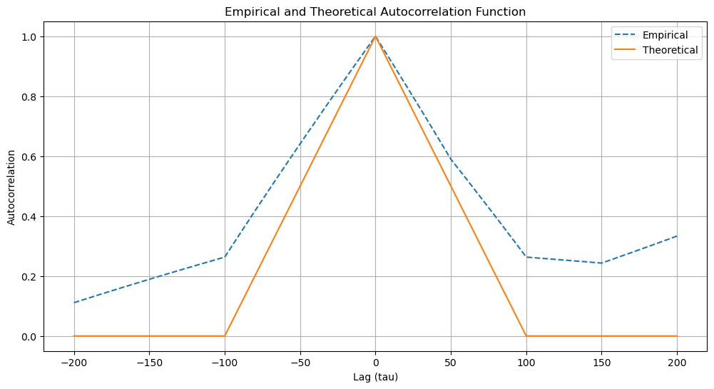
Combining the results, the autocorrelation function is:
# Compute empirical autocorrelation
def empirical_autocorrelation(x_t, tau_values):
    autocorr = []
    N = len(x_t)
    for tau in tau_values:
        if tau < 0:
            x_t_tau = np.roll(x_t, tau)
            autocorr.append(np.dot(x_t[:N+tau], x_t_tau[:N+tau]) / (N+tau))
        else:
            x_t_tau = np.roll(x_t, -tau)
            autocorr.append(np.dot(x_t[tau:], x_t_tau[tau:]) / (N-tau))
    return np.array(autocorr)

# Define tau values for which to calculate autocorrelation
max_tau = T_c * 2
tau_values = np.arange(-max_tau, max_tau + 1)

# Calculate empirical autocorrelation
empirical_Rx = empirical_autocorrelation(x_t, tau_values)

# Theoretical autocorrelation function
def theoretical_autocorrelation(tau, T_c):
    return np.where(np.abs(tau) <= T_c, 1 - np.abs(tau) / T_c, 0)

theoretical_Rx = theoretical_autocorrelation(tau_values, T_c)

# Plot empirical and theoretical autocorrelation functions
plt.figure(figsize=(12, 6))
plt.plot(tau_values, empirical_Rx, label='Empirical', linestyle='--')
plt.plot(tau_values, theoretical_Rx, label='Theoretical')
plt.xlabel('Lag (tau)')
plt.ylabel('Autocorrelation')
plt.title('Empirical and Theoretical Autocorrelation Function')
plt.legend()
plt.grid(True)
plt.show()
Power Spectral Density (PSD)#
The power spectral density (PSD) is a crucial tool in the analysis of stochastic processes, especially for stationary processes. It provides insight into how the power of a signal or time series is distributed over different frequency components.
Continuous Stationary Process#
For a continuous stationary process, the PSD describes the distribution of power over frequency. Here are the detailed steps and formulas:
Definition of PSD#
Autocorrelation Function: The autocorrelation function \( R(\tau) \) of a continuous stationary process is defined as:
\[ R(\tau) = E\{\mathbf{x}(t) \mathbf{x}(t + \tau)\} \]where \( E \{\cdot\} \) denotes the expectation operator, and \( \tau \) is the time lag.
PSD via Fourier Transform: The PSD \( S(f) \) is obtained by taking the Fourier transform of the autocorrelation function \( R(\tau) \):
\[ S(f) = \int_{-\infty}^{\infty} R(\tau) e^{-j2\pi f \tau} \, d\tau \]Here, \( f \) represents the frequency, and \( j \) is the imaginary unit.
Inverse Relationship#
Inverse Fourier Transform: Conversely, the autocorrelation function \( R(\tau) \) can be retrieved from the PSD \( S(f) \) using the inverse Fourier transform:
\[ R(\tau) = \int_{-\infty}^{\infty} S(f) e^{j2\pi f \tau} \, df \]This shows that the autocorrelation function and the PSD are a Fourier transform pair.
Properties and Implications#
Stationarity: For a process to be stationary, the statistical properties, including the autocorrelation function, do not change with time shifts.
Spectral Representation: The PSD provides a frequency domain representation of the process, highlighting the contribution of different frequencies to the overall power.
Discrete Stationary Process#
For a discrete stationary process, the concepts are similar but involve summations instead of integrals.
Definition of PSD#
Autocorrelation Function: The autocorrelation function \( R(n) \) of a discrete stationary process \(\{\mathbf{x}(n)\}\) is defined as:
\[ R(n) = E\{\mathbf{x}(m) \mathbf{x}(m + n)\} \]where \( n \) is an integer time lag.
PSD via Discrete-Time Fourier Transform: The PSD \( S(f) \) is given by the discrete-time Fourier transform (DTFT) of the autocorrelation function \( R(n) \):
\[ S(f) = \sum_{n=-\infty}^{\infty} R(n) e^{-j2\pi f n} \]Here, \( f \) is a normalized frequency.
Inverse Relationship#
Inverse DTFT: The autocorrelation function \( R(n) \) can be retrieved from the PSD \( S(f) \) using the inverse DTFT:
\[ R(n) = \int_{-\infty}^{\infty} S(f) e^{j2\pi f n} \, df \]
Properties and Implications#
Stationarity: Similar to the continuous case, the statistical properties of a discrete stationary process do not change over time.
Spectral Representation: The PSD in the discrete case provides a frequency domain representation that shows how power is distributed among different frequency components of the discrete process.
Example: PSD of a Random Square Wave#
In this example, continuing from the previous example, we will now derive and understand the power spectral density (PSD) of the random square wave process \(\mathbf{x}(t)\).
We previously derived the autocorrelation function for the random square wave process as:
The PSD \( S_{\mathbf{x}}(f) \) is obtained by taking the Fourier transform of the autocorrelation function \( R_{\mathbf{x}}(\tau) \):
Given the symmetry and the fact that \( R_{\mathbf{x}}(\tau) \) is zero for \( |\tau| > T_c \), the integral can be simplified and evaluated over the interval \([-T_c, T_c]\):
Using the given integral, we have
Using integration by parts and properties of trigonometric integrals, we have
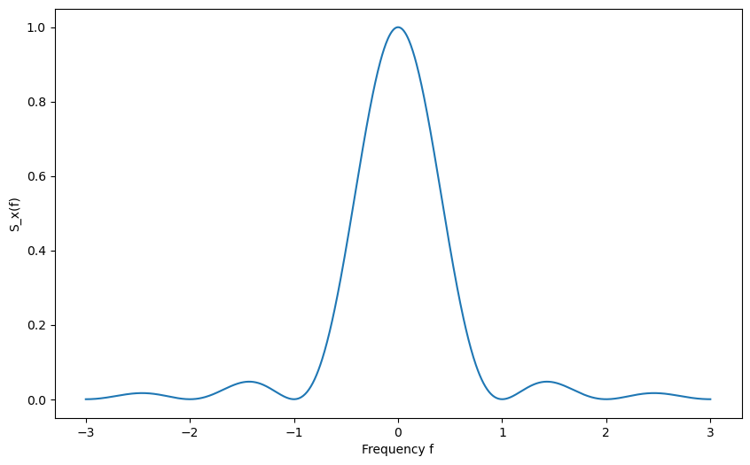
Using trigonometric identities, the expression can be further simplified to:
import numpy as np
import matplotlib.pyplot as plt

def theoretical_psd(f, Tc):
    """Compute the theoretical PSD of a random square wave."""
    return Tc * (np.sin(np.pi * f * Tc) / (np.pi * f * Tc))**2

# Parameters
Tc = 1  # Period of the square wave
f_limit = 3 / Tc  # Frequency limit for plotting

# Frequency range
f = np.linspace(-f_limit, f_limit, 1000)

# Compute theoretical PSD
psd_theoretical = theoretical_psd(f, Tc)

# Plot the theoretical PSD
plt.figure(figsize=(10, 6))
plt.plot(f, psd_theoretical, label="Theoretical PSD")
plt.xlabel('Frequency f')
plt.ylabel('S_x(f)')
Text(0, 0.5, 'S_x(f)')
Note: this simulation is not 100% correct, there is still a small misalligment between empirical and theoretical PSD.
import numpy as np
import matplotlib.pyplot as plt
from scipy.fft import fft, fftfreq, fftshift

def generate_random_square_wave(t, Tc, dt):
    """Generate a random square wave with period Tc."""
    n_intervals = len(t) // int(Tc / dt)
    wave = np.repeat(np.random.choice([1, -1], n_intervals), int(Tc / dt))
    return wave[:len(t)]

def theoretical_psd(f, Tc):
    """Compute the theoretical PSD of a random square wave."""
    return Tc * (np.sin(np.pi * f * Tc) / (np.pi * f * Tc))**2

# Parameters
Tc = 1  # Period of the square wave
T = 100  # Total time duration
dt = 0.001  # Time step
t = np.arange(0, T, dt)
N = len(t)  # Number of samples

# Generate random square wave
x = generate_random_square_wave(t, Tc, dt)

# Compute empirical PSD using FFT
X = fft(x)
psd_empirical = (np.abs(X) ** 2) / (N * dt)
frequencies = fftfreq(N, dt)

# Shift the PSD and frequency vectors for proper display
psd_empirical_shifted = fftshift(psd_empirical)
frequencies_shifted = fftshift(frequencies)

# Normalize both PSDs
psd_empirical_shifted /= np.max(psd_empirical_shifted)

# Limit the frequency range to around ±3/Tc
freq_limit = 3 / Tc
indices = np.where(np.abs(frequencies_shifted) <= freq_limit)
frequencies_shifted = frequencies_shifted[indices]
psd_empirical_shifted = psd_empirical_shifted[indices]

# Compute theoretical PSD
psd_theoretical = theoretical_psd(frequencies_shifted, Tc)

# Plot the random square wave
plt.figure(figsize=(14, 3))

plt.plot(t, x, label="Random Square Wave")
plt.xlabel('Time t')
plt.ylabel('x(t)')
plt.title('Random Square Wave Signal')
plt.legend()
plt.grid(True)

plt.figure(figsize=(14, 6))

# Plot the empirical and theoretical PSD
plt.plot(frequencies_shifted, psd_empirical_shifted, label="Empirical PSD")
plt.xlabel('Frequency f')
plt.ylabel('S_x(f)')
plt.title('Empirical Power Spectral Density')
plt.legend()
plt.grid(True)

plt.plot(frequencies_shifted, psd_theoretical, label="Theoretical PSD", linestyle='dashed')
plt.xlabel('Frequency f')
plt.ylabel('S_x(f)')
plt.title('Theoretical Power Spectral Density')
plt.legend()
plt.grid(True)

plt.tight_layout()
plt.show()

# Convert PSD to dB scale
psd_empirical_shifted_db = 10 * np.log10(psd_empirical_shifted)
psd_theoretical_db = 10 * np.log10(psd_theoretical)

# Plot the random square wave
plt.figure(figsize=(14, 8))

# Plot the empirical PSD in dB scale
plt.plot(frequencies_shifted, psd_empirical_shifted_db, label="Empirical PSD (dB)")
plt.xlabel('Frequency f')
plt.ylabel('S_x(f) (dB)')
plt.title('Empirical Power Spectral Density (dB)')
plt.legend()
plt.grid(True)

plt.plot(frequencies_shifted, psd_theoretical_db, label="Theoretical PSD (dB)", linestyle='dashed')
plt.xlabel('Frequency f')
plt.ylabel('S_x(f) (dB)')
plt.title('Theoretical Power Spectral Density (dB)')
plt.legend()
plt.grid(True)

plt.tight_layout()
plt.show()

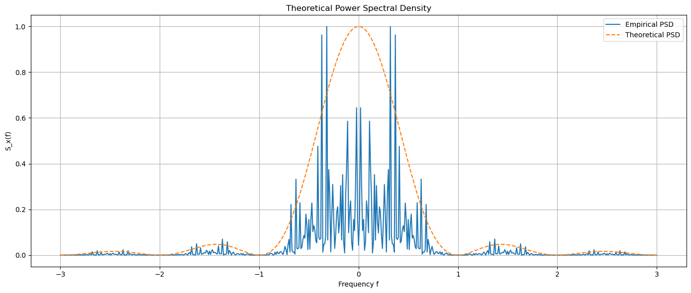
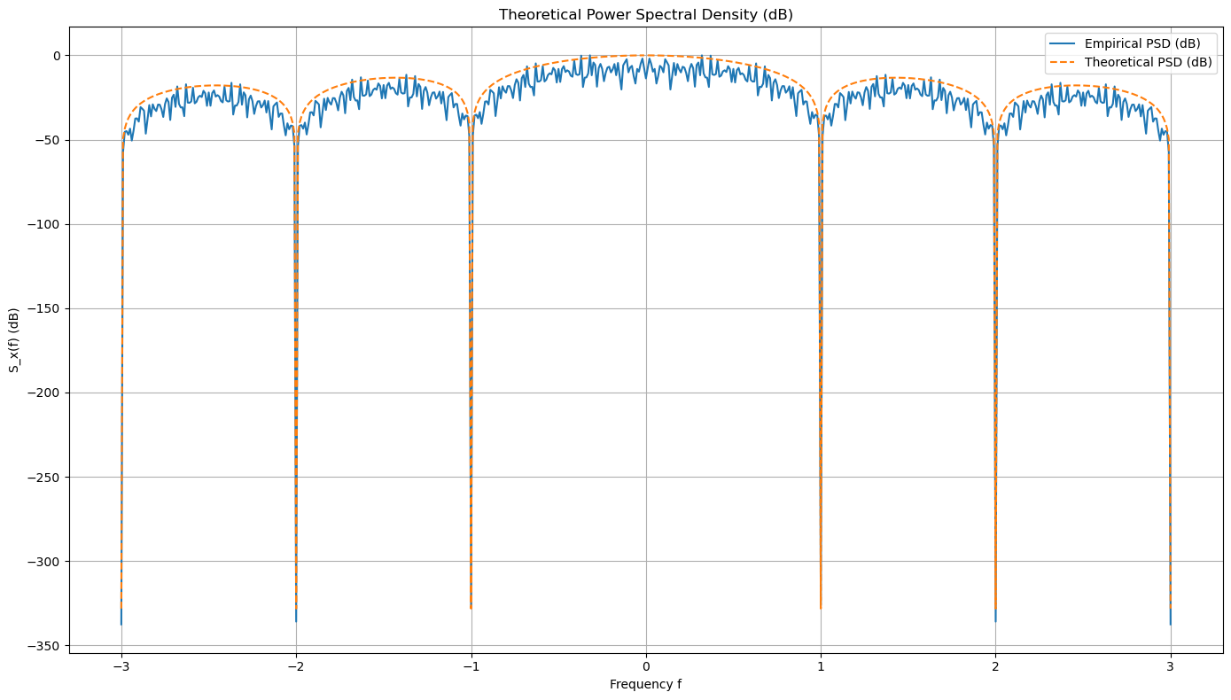
Note: we must use fftshift to obtain correct PSD in dB scale.
fftshift is not strictly necessary, but it helps to center the zero frequency component, making the PSD plot easier to interpret. The zero frequency (DC component) is placed in the middle of the frequency axis, allowing for a symmetrical view of both positive and negative frequencies.
Ergodicity#
Ergodicity in Stationary Processes#
Ergodicity is a fundamental concept in the study of stochastic processes, particularly stationary processes. A stationary process is one whose statistical properties do not change over time. Specifically, ergodicity implies that time averages of the process converge to the ensemble averages. This means that the statistical properties of a single time series realization of the process can represent the entire ensemble of possible realizations.
Mathematical Definition#
For a stationary process \(\mathbf{x}(t)\), ergodicity is mathematically expressed as:
Here, \(E\{\mathbf{x}^m(t_1)\}\) denotes the ensemble average, and the integral on the right-hand side represents the time average over a period \([-T, T]\).
Practical Implications#
Single Realization Sufficiency:
For an ergodic process, the statistical properties (such as mean, variance) and power spectral density can be accurately determined from a single, sufficiently long realization of the process.
Ergodicity in the Mean:
A process is ergodic in the mean if the above relation holds for \(m = 1\). This means that the time average of the process converges to its mean over an infinite time horizon.
Conditions for Ergodicity in the Mean:
For a stationary process to be ergodic in the mean, it must satisfy the following condition:
\[ \lim_{T \to \infty} \frac{1}{T} \int_0^T (R(\tau) - \mu^2) d\tau = 0 \]where \(R(\tau)\) is the autocorrelation function of the process, and \(\mu\) is the mean of the process. This condition ensures that the deviations from the mean over time diminish as the observation period becomes infinitely long.
Challenges and Assumptions#
Demonstrating Complete Ergodicity:
Proving ergodicity rigorously for a given process can be challenging due to the complexity involved in establishing the convergence of time averages to ensemble averages.
Assumptions in Practice:
Despite the difficulty in proving ergodicity, it is often assumed in practical applications. This assumption simplifies the analysis and allows for the use of time averages to estimate statistical properties.
Example: Ergodicity of a Random Square Wave#
To mathematically test if the described process is ergodic, we need to verify that its time averages converge to its ensemble averages. We will do this by checking two primary conditions:
Mean Ergodicity: Verify if the time average of the process converges to its mean.
Autocorrelation Function: Verify if the time-averaged autocorrelation function converges to the ensemble-averaged autocorrelation function.
Mean Ergodicity#
For a process to be mean ergodic, the time average should equal the ensemble average.
Mean of the Process#
Given that the process \(\mathbf{x}(t)\) takes values \(+1\) and \(-1\) with equal probability, the ensemble mean \(\mu\) is:
Time Average of the Process#
The time average \(\bar{x}_T\) over an interval \([-T, T]\) is given by:
For ergodicity in the mean, we need:
Since \(\mathbf{x}(t)\) alternates between \(+1\) and \(-1\) with equal probability over sufficiently large intervals, the positive and negative contributions should cancel out, making \(\bar{x}_T\) approach 0 as \(T \to \infty\).
Autocorrelation Function Ergodicity#
Next, we consider the autocorrelation function \(R(\tau)\). For ergodicity, the time-averaged autocorrelation should converge to the ensemble-averaged autocorrelation.
Autocorrelation Function#
The ensemble autocorrelation function is:
For our random square wave:
\(R(0) = E[\mathbf{x}(t)^2] = 1\)
For \(\tau \neq 0\), since \(\mathbf{x}(t)\) and \(\mathbf{x}(t + \tau)\) are uncorrelated over different \(T_c\) intervals, \(R(\tau) = 0\)
Hence, the autocorrelation function is:
Time-Averaged Autocorrelation Function#
The time-averaged autocorrelation function over an interval \([0, T]\) is:
For the process to be ergodic in the autocorrelation function, we need:
Since the process is uncorrelated over different \(T_c\) intervals, \(\hat{R}_T(\tau)\) should also approach the ensemble average \(R(\tau)\).
