Zero Mean Complex Circularly Symmetric Gaussian (ZMCCSG) RV#
A Zero Mean Complex Circularly Symmetric Gaussian (ZMCCSG) random variable (RV) is a fundamental concept in wireless communications and signal processing, particularly in the analysis and modeling of noise and signals in complex domains.
Consider a complex RV \(\mathbf{x}\) defined as follows:
where:
\(\mathbf{x}_R\) is the real part of the RV \(\mathbf{x}\).
\(\mathbf{x}_I\) is the imaginary part of the RV \(\mathbf{x}\).
\(j\) denotes the imaginary unit (i.e., \(j = \sqrt{-1}\)).
Properties of \(\mathbf{x}_R\) and \(\mathbf{x}_I\)#
\(\mathbf{x}_R\) and \(\mathbf{x}_I\) are independent and identically distributed (iid).
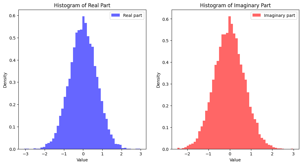
Both \(\mathbf{x}_R\) and \(\mathbf{x}_I\) are normally distributed with mean zero and variance \(\frac{\sigma^2}{2}\). Thus, \(\mathbf{x}_R \sim \mathcal{N}(0, \frac{\sigma^2}{2})\) and \(\mathbf{x}_I \sim \mathcal{N}(0, \frac{\sigma^2}{2})\).
Because \(\mathbf{x}_R\) and \(\mathbf{x}_I\) are iid normal random variables, their joint distribution defines \(\mathbf{x}\) as a complex Gaussian RV.
Complex Circular Symmetry#
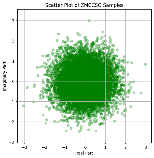
A complex RV \(\mathbf{x}\) is said to be circularly symmetric if its statistical properties are invariant to multiplication by a complex exponential of any phase \(\theta\). Mathematically, this means that for any \(\theta\):
where \(\stackrel{d}{=}\) denotes equality in distribution.
This property implies that the magnitude and phase of \(\mathbf{x}\) are independent, with the phase uniformly distributed over \([0, 2\pi)\) and the magnitude having a Rayleigh distribution.
Zero Mean and Variance#
The term “zero mean” indicates that the expected value of \(\mathbf{x}\) is zero:
The variance \(\sigma^2\) of the complex RV \(\mathbf{x}\) is the total variance, which includes contributions from both the real and imaginary parts. Given the variances of \(\mathbf{x}_R\) and \(\mathbf{x}_I\), the total variance \(\sigma^2\) is:
Thus, we denote this ZMCCSG RV as \(\mathbf{x} \sim \mathcal{CN}(0, \sigma^2)\).
Standard ZMCCSG Random Variable#
A standard ZMCCSG RV \(\mathbf{w}\) is a special case where the variance \(\sigma^2\) is set to 1. Hence, the real and imaginary parts of \(\mathbf{w}\) are iid normal random variables with zero mean and variance \(\frac{1}{2}\):
This leads to:
Summary
A Zero Mean Complex Circularly Symmetric Gaussian (ZMCCSG) RV \(\mathbf{x}\) is defined as a complex RV with its real and imaginary parts being independent, identically distributed normal random variables with zero mean and equal variance. The RV has zero mean and a specified total variance \(\sigma^2\). This concept is fundamental in modeling complex noise and signal processes in various fields of engineering and science.
import numpy as np
import matplotlib.pyplot as plt
import warnings
warnings.filterwarnings("ignore")

# Function to generate ZMCCSG random variable
def generate_zmccsg(n_samples, sigma):
    # Generate real and imaginary parts independently
    x_R = np.random.normal(0, sigma / np.sqrt(2), n_samples)
    x_I = np.random.normal(0, sigma / np.sqrt(2), n_samples)

    # Combine real and imaginary parts to form the complex random variable
    x = x_R + 1j * x_I

    return x

# Parameters
n_samples = 10000
sigma = 1  # Standard deviation of the ZMCCSG random variable

# Generate ZMCCSG random variable
zmccsg_samples = generate_zmccsg(n_samples, sigma)

# Plot the real and imaginary parts
plt.figure(figsize=(12, 6))

plt.subplot(1, 2, 1)
plt.hist(np.real(zmccsg_samples), bins=50, density=True, alpha=0.6, color='b', label='Real part')
plt.title('Histogram of Real Part')
plt.xlabel('Value')
plt.ylabel('Density')
plt.legend()

plt.subplot(1, 2, 2)
plt.hist(np.imag(zmccsg_samples), bins=50, density=True, alpha=0.6, color='r', label='Imaginary part')
plt.title('Histogram of Imaginary Part')
plt.xlabel('Value')
plt.ylabel('Density')
plt.legend()

plt.show()

# Plot the complex plane
plt.figure(figsize=(6, 6))
plt.scatter(np.real(zmccsg_samples), np.imag(zmccsg_samples), alpha=0.3, color='g')
plt.title('Scatter Plot of ZMCCSG Samples')
plt.xlabel('Real Part')
plt.ylabel('Imaginary Part')
plt.axis('equal')
plt.grid(True)
plt.show()


import numpy as np
import matplotlib.pyplot as plt

# Function to generate ZMCCSG random variable
def generate_zmccsg(n_samples, sigma):
    # Generate real and imaginary parts independently
    x_R = np.random.normal(0, sigma / np.sqrt(2), n_samples)
    x_I = np.random.normal(0, sigma / np.sqrt(2), n_samples)

    # Combine real and imaginary parts to form the complex random variable
    x = x_R + 1j * x_I

    return x

# Parameters
n_samples = 10000
sigma = 1  # Standard deviation of the ZMCCSG random variable

# Generate ZMCCSG random variable
w = generate_zmccsg(n_samples, sigma)

# Compute phase and magnitude
phases = np.angle(w)
magnitudes = np.abs(w)
magnitude_squared = magnitudes**2

# Plot the phase distribution
plt.figure(figsize=(18, 6))

plt.subplot(1, 3, 1)
plt.hist(phases, bins=50, density=True, alpha=0.6, color='b', label='Empirical Phase')
# Theoretical uniform distribution for phase
uniform_phase = np.ones_like(phases) / (2 * np.pi)
plt.plot(np.linspace(-np.pi, np.pi, 1000), uniform_phase[:1000], 'r--', label='Theoretical Uniform PDF')
plt.title('Histogram of Phase')
plt.xlabel('Phase (radians)')
plt.ylabel('Density')
plt.legend()

# Plot the magnitude distribution
# Rayleigh distribution parameter : sigma / np.sqrt(2)
plt.subplot(1, 3, 2)
plt.hist(magnitudes, bins=50, density=True, alpha=0.6, color='g', label='Empirical Magnitude')
r = np.linspace(0, 4*sigma, 1000)
theoretical_rayleigh = (r / (sigma / np.sqrt(2))**2) * np.exp(-r**2 / (2 * (sigma / np.sqrt(2))**2))
plt.plot(r, theoretical_rayleigh, 'k--', label='Theoretical Rayleigh PDF')
plt.title('Histogram of Magnitude')
plt.xlabel('Magnitude')
plt.ylabel('Density')
plt.legend()

# Plot the magnitude squared distribution
plt.subplot(1, 3, 3)
plt.hist(magnitude_squared, bins=50, density=True, alpha=0.6, color='r', label='Empirical Magnitude Squared')
x = np.linspace(0, 4*sigma**2, 1000)
theoretical_exponential = (1 / sigma**2) * np.exp(-x / sigma**2)
plt.plot(x, theoretical_exponential, 'k--', label='Theoretical Exponential PDF')
plt.title('Histogram of Magnitude Squared')
plt.xlabel('Magnitude Squared')
plt.ylabel('Density')
plt.legend()

plt.tight_layout()
plt.show()

Derivation of the Rayleigh Distribution#
To demonstrate that the magnitude \( |\mathbf{x}_R + j \mathbf{x}_I| \) follows the Rayleigh distribution, we begin with the following components:
\( \mathbf{x}_R \sim \mathcal{N} \left(0, \frac{\sigma^2}{2} \right) \): a normally distributed RV with mean 0 and variance \( \frac{\sigma^2}{2} \).
\( \mathbf{x}_I \sim \mathcal{N} \left( 0, \frac{\sigma^2}{2} \right) \): another normally distributed RV with mean 0 and variance \( \frac{\sigma^2}{2} \).
We form the complex RV \( \mathbf{x} = \mathbf{x}_R + j \mathbf{x}_I \), where \( j \) is the imaginary unit.
The magnitude \( \mathbf{r} \) of the complex number \( \mathbf{x} \) is defined as:
Since both \( \mathbf{x}_R \) and \( \mathbf{x}_I \) are independent and normally distributed with zero mean and variance \( \frac{\sigma^2}{2} \), the sum of their squares, \( r^2 = \mathbf{x}_R^2 + \mathbf{x}_I^2 \), follows a chi-squared distribution with 2 degrees of freedom. This distribution can also be viewed as a gamma distribution with shape parameter \( k = 1 \) and scale parameter \( \theta = \frac{\sigma^2}{2} \).
The probability density function (PDF) of \( r^2 \) is:
To derive the PDF of \( \mathbf{r} \), we utilize the transformation relationship between \( \mathbf{r} \) and \( \mathbf{r}^2 \):
where \( r \) and \( r^2 \) are realizations of \( \mathbf{r} \) and \( \mathbf{r}^2 \).
Let \( g(r^2) = \sqrt{r^2} \) and its inverse \( g^{-1}(r) = r^2 \).
The Jacobian determinant of this transformation is given by:
Thus, the PDF of \( \mathbf{r} \), denoted as \( f_{\mathbf{r}}(r) \), is obtained by transforming the PDF of \( r^2 \) using the Jacobian determinant:
Substituting the expressions, we get:
This is the Rayleigh distribution with the scale parameter \( \sigma' = \frac{\sigma}{\sqrt{2}} \).
Thus, the magnitude \( |\mathbf{x}_R + j \mathbf{x}_I| \) indeed follows the Rayleigh distribution. The PDF of the magnitude \( \mathbf{r} \) can be expressed as:
where \( \sigma' = \frac{\sigma}{\sqrt{2}} \).
This result confirms that the magnitude of a complex number, whose real and imaginary components are independent and identically distributed normal random variables, follows the Rayleigh distribution.
Derivation of the Exponential Distribution#
To prove that the magnitude squared of a complex Gaussian RV follows an exponential distribution, we start with the following:
For a complex RV \( \mathbf{x} = \mathbf{x}_R + j \mathbf{x}_I \), where \( \mathbf{x}_R \) and \( \mathbf{x}_I \) are independent and normally distributed with mean 0 and variance \( \frac{\sigma^2}{2} \), the magnitude squared is given by:
This can be expressed as:
where \( \mathbf{z} \sim \chi^2_2 \), a chi-squared distribution with 2 degrees of freedom. The chi-squared distribution with 2 degrees of freedom is equivalent to a gamma distribution with shape parameter \( k = 1 \) and scale parameter \( \theta = 2 \), denoted as \( \Gamma(k=1, \theta=2) \). This gamma distribution is also equivalent to an exponential distribution with rate parameter \( \lambda = \frac{1}{2} \).
Thus, \( \mathbf{z} \) can be represented as an exponential random variable:
The PDF of \( \mathbf{z} \) is given by:
To find the PDF of \( \mathbf{y} = |\mathbf{x}|^2 = \frac{\sigma^2}{2} \mathbf{z} \), we use the transformation technique. The relationship between \( \mathbf{y} \) and \( \mathbf{z} \) is:
To find the PDF of \( \mathbf{y} \), we use the formula for transforming the PDF under a change of variables:
Substituting \( f_{\mathbf{z}}(z) \) and calculating the derivative, we obtain:
Thus, the magnitude squared \( |\mathbf{x}|^2 \) follows an exponential distribution with the PDF:
This shows that the magnitude squared of a complex Gaussian random variable, where the real and imaginary parts are independent and identically distributed normal random variables, follows an exponential distribution with parameter \( \frac{1}{\sigma^2} \).
