Complex Random Variables#
In communication systems, baseband representation is a fundamental concept, allowing the simplification of signal processing tasks by focusing on the frequency components near zero frequency. This approach often involves the use of complex random vectors to model and analyze the behavior of signals.
Definition of a Complex Random Vector#
A complex random vector \(\vec{\mathbf{x}}\) can be expressed as:
Here:
\(\vec{\mathbf{x}}_R\) is the real part of the complex random vector, a real-valued random vector.
\(\vec{\mathbf{x}}_I\) is the imaginary part of the complex random vector, also a real-valued random vector.
\(j\) is the imaginary unit, satisfying \(j^2 = -1\).
This decomposition into real and imaginary parts is crucial because it allows the use of real-valued statistical techniques and tools to analyze complex signals.
Circular Symmetry#
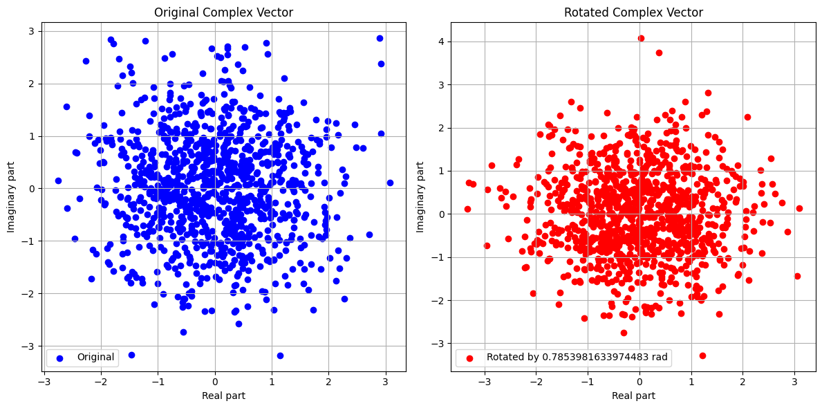
In the context of communication systems, a key property of complex random vectors is circular symmetry. A complex random vector \(\vec{\mathbf{x}}\) is said to be circularly symmetric if its statistical properties are invariant under phase rotations. Mathematically, this means:
This notation indicates that the distribution of the vector \(\vec{\mathbf{x}}\) remains the same regardless of the phase shift \(\theta\). Here, \(\sim\) denotes equality in distribution.
Circular symmetry is an important property because many natural and man-made signals exhibit this characteristic, simplifying the analysis and processing of these signals.
Statistical Characterization#
The first and second-order statistics of a circularly symmetric complex random vector can provide comprehensive information about the vector. Specifically, these statistics are characterized by the expected value and the covariance matrix.
Mean (First-Order Statistics):
The mean of \(\vec{\mathbf{x}}\) is defined as:
For a circularly symmetric vector, the mean is often zero (i.e., \( E[\vec{\mathbf{x}}] = \vec{0} \)).
Covariance Matrix (Second-Order Statistics):
The second-order statistics are encapsulated in the covariance matrix, given by:
Here:
\(E[\cdot]\) denotes the expectation operator.
\((\cdot)^{\mathsf{H}}\) denotes the Hermitian transpose (conjugate transpose).
The covariance matrix provides information about the power and correlation of the components of the vector \(\vec{\mathbf{x}}\).
import numpy as np
import matplotlib.pyplot as plt
import warnings
warnings.filterwarnings("ignore")

# Function to generate a circularly symmetric complex random vector
def generate_complex_random_vector(n):
    real_part = np.random.normal(size=n)
    imag_part = np.random.normal(size=n)
    complex_vector = real_part + 1j * imag_part
    return complex_vector

# Function to rotate the complex vector by a phase angle theta
def rotate_vector(vector, theta):
    return np.exp(1j * theta) * vector

# Function to plot the real and imaginary parts of the vectors
def plot_vectors(original, rotated, theta):
    plt.figure(figsize=(12, 6))

    plt.subplot(1, 2, 1)
    plt.scatter(original.real, original.imag, color='blue', label='Original')
    plt.xlabel('Real part')
    plt.ylabel('Imaginary part')
    plt.title('Original Complex Vector')
    plt.grid(True)
    plt.legend()

    plt.subplot(1, 2, 2)
    plt.scatter(rotated.real, rotated.imag, color='red', label=f'Rotated by {theta} rad')
    plt.xlabel('Real part')
    plt.ylabel('Imaginary part')
    plt.title('Rotated Complex Vector')
    plt.grid(True)
    plt.legend()

    plt.tight_layout()
    plt.show()

# Parameters
n = 1000  # Size of the complex random vector
theta = np.pi / 4  # Rotation angle (45 degrees)

# Generate the complex random vector
complex_vector = generate_complex_random_vector(n)

# Rotate the vector by theta
rotated_vector = rotate_vector(complex_vector, theta)

# Plot the original and rotated vectors
plot_vectors(complex_vector, rotated_vector, theta)

# Calculate and compare statistical properties
original_mean = np.mean(complex_vector)
original_variance = np.var(complex_vector)

rotated_mean = np.mean(rotated_vector)
rotated_variance = np.var(rotated_vector)

print(f"Original Mean: {original_mean}")
print(f"Rotated Mean: {rotated_mean}")
print(f"Original Variance: {original_variance}")
print(f"Rotated Variance: {rotated_variance}")

# Check if the distributions are similar
mean_diff = np.abs(original_mean - rotated_mean)
variance_diff = np.abs(original_variance - rotated_variance)

print(f"Difference in Mean: {mean_diff}")
print(f"Difference in Variance: {variance_diff}")

Original Mean: (0.0053185447225258305+0.038816542741353585j)
Rotated Mean: (-0.023686661555286623+0.031208219633970514j)
Original Variance: 2.0640208274427003
Rotated Variance: 2.0640208274427003
Difference in Mean: 0.029986473145816768
Difference in Variance: 0.0
Discussion on Circularly Symmetric Property#
A random vector \( \vec{\mathbf{x}} \) is said to be circularly symmetric if its distribution remains unchanged under multiplication by \( e^{j\theta} \) for any real \( \theta \). Mathematically, this can be expressed as:
where \( \overset{d}{=} \) denotes equality in distribution.
Rotation in the Complex Plane#
In the complex plane, rotating \( \vec{\mathbf{x}} \) by an angle \( \theta \) is equivalent to multiplying \( \vec{\mathbf{x}} \) by \( e^{j\theta} \), a complex number of unit magnitude.
Equality in Distribution#
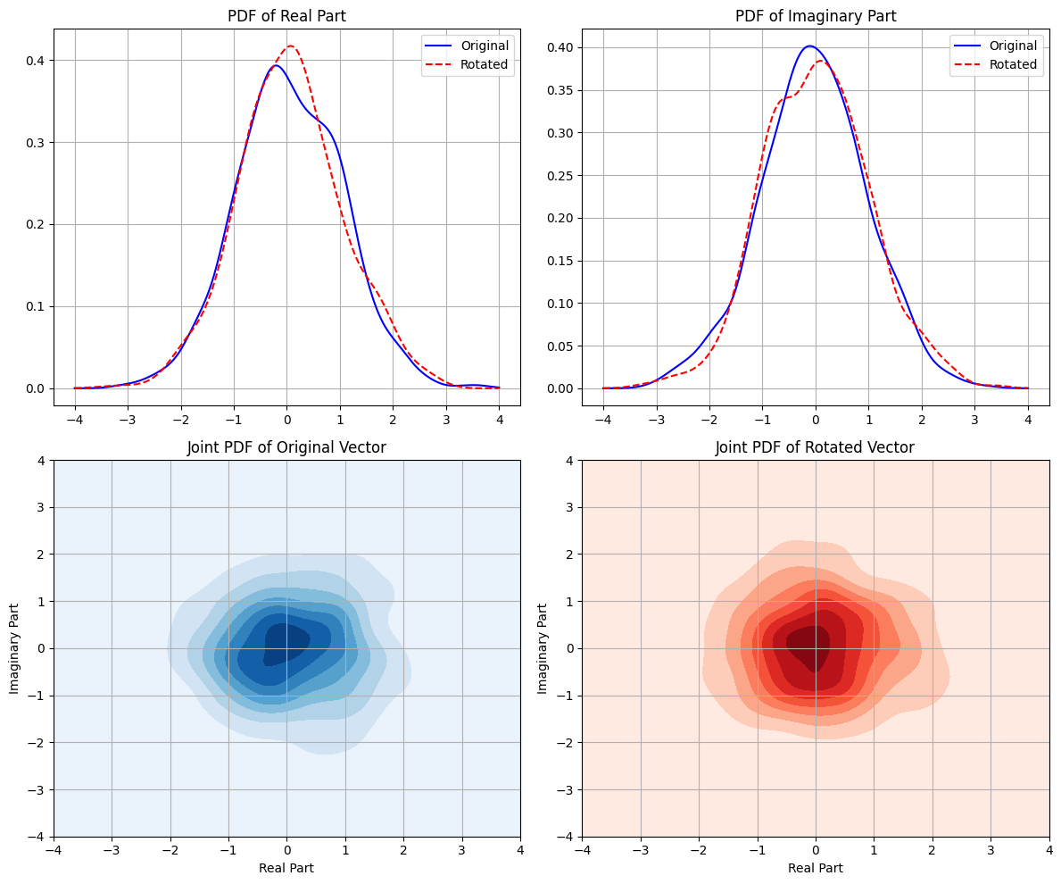
The condition \( e^{j\theta}\vec{\mathbf{x}} \sim \vec{\mathbf{x}} \) implies that the random vector \( \vec{\mathbf{x}} \) and its rotated version \( e^{j\theta}\vec{\mathbf{x}} \) have the same probability distribution.
Implications#
For \( \vec{\mathbf{x}} \) to be circularly symmetric, the joint distribution of its real and imaginary parts must be identical to that of the rotated vector.
This requirement implies that both the mean vector and the covariance matrix of \( \vec{\mathbf{x}} \) must be invariant under rotation.
Covariance Matrix#
Denoting the covariance matrix of \( \vec{\mathbf{x}} \) by \( \Sigma \), for \( \vec{\mathbf{x}} \) to be circularly symmetric, \( \Sigma \) must satisfy:
where \( R_\theta \) is the rotation matrix given by:
Invariant Covariance#
The condition above implies that \( \Sigma \) must be proportional to the identity matrix, as only a scaled identity matrix is invariant under all rotations. Thus, we have:
where \( \sigma^2 \) is a positive constant and \( I \) is the identity matrix.
Since the covariance matrix \( \Sigma \) is proportional to the identity matrix, the random vector \( \vec{\mathbf{x}} \) has the same distribution as its rotated version, confirming that \( \vec{\mathbf{x}} \) is circularly symmetric.
import numpy as np
import matplotlib.pyplot as plt
from scipy.stats import gaussian_kde

# Function to generate a circularly symmetric complex random vector
def generate_complex_random_vector(n):
    real_part = np.random.normal(size=n)
    imag_part = np.random.normal(size=n)
    complex_vector = real_part + 1j * imag_part
    return complex_vector

# Function to rotate the complex vector by a phase angle theta
def rotate_vector(vector, theta):
    return np.exp(1j * theta) * vector

# Function to plot the PDFs of the original and rotated vectors
def plot_pdfs(original, rotated):
    fig, axs = plt.subplots(2, 2, figsize=(12, 10))

    # Real part PDF
    kde_original_real = gaussian_kde(original.real)
    kde_rotated_real = gaussian_kde(rotated.real)
    x_real = np.linspace(-4, 4, 1000)
    axs[0, 0].plot(x_real, kde_original_real(x_real), color='blue', label='Original')
    axs[0, 0].plot(x_real, kde_rotated_real(x_real), color='red', linestyle='--', label='Rotated')
    axs[0, 0].set_title('PDF of Real Part')
    axs[0, 0].legend()
    axs[0, 0].grid(True)

    # Imaginary part PDF
    kde_original_imag = gaussian_kde(original.imag)
    kde_rotated_imag = gaussian_kde(rotated.imag)
    x_imag = np.linspace(-4, 4, 1000)
    axs[0, 1].plot(x_imag, kde_original_imag(x_imag), color='blue', label='Original')
    axs[0, 1].plot(x_imag, kde_rotated_imag(x_imag), color='red', linestyle='--', label='Rotated')
    axs[0, 1].set_title('PDF of Imaginary Part')
    axs[0, 1].legend()
    axs[0, 1].grid(True)

    # Joint PDF of Real and Imaginary parts for Original Vector
    kde_original_joint = gaussian_kde([original.real, original.imag])
    x, y = np.mgrid[-4:4:100j, -4:4:100j]
    positions = np.vstack([x.ravel(), y.ravel()])
    z_original = np.reshape(kde_original_joint(positions).T, x.shape)
    axs[1, 0].contourf(x, y, z_original, cmap='Blues')
    axs[1, 0].set_title('Joint PDF of Original Vector')
    axs[1, 0].set_xlabel('Real Part')
    axs[1, 0].set_ylabel('Imaginary Part')
    axs[1, 0].grid(True)

    # Joint PDF of Real and Imaginary parts for Rotated Vector
    kde_rotated_joint = gaussian_kde([rotated.real, rotated.imag])
    z_rotated = np.reshape(kde_rotated_joint(positions).T, x.shape)
    axs[1, 1].contourf(x, y, z_rotated, cmap='Reds')
    axs[1, 1].set_title('Joint PDF of Rotated Vector')
    axs[1, 1].set_xlabel('Real Part')
    axs[1, 1].set_ylabel('Imaginary Part')
    axs[1, 1].grid(True)

    plt.tight_layout()
    plt.show()

# Parameters
n = 1000  # Size of the complex random vector
theta = np.pi / 4  # Rotation angle (45 degrees)

# Generate the complex random vector
complex_vector = generate_complex_random_vector(n)

# Rotate the vector by theta
rotated_vector = rotate_vector(complex_vector, theta)

# Plot the PDFs of the original and rotated vectors
plot_pdfs(complex_vector, rotated_vector)

# Calculate and compare statistical properties
original_mean = np.mean(complex_vector)
original_variance = np.var(complex_vector)

rotated_mean = np.mean(rotated_vector)
rotated_variance = np.var(rotated_vector)

print(f"Original Mean: {original_mean}")
print(f"Rotated Mean: {rotated_mean}")
print(f"Original Variance: {original_variance}")
print(f"Rotated Variance: {rotated_variance}")

# Check if the distributions are similar
mean_diff = np.abs(original_mean - rotated_mean)
variance_diff = np.abs(original_variance - rotated_variance)

print(f"Difference in Mean: {mean_diff}")
print(f"Difference in Variance: {variance_diff}")

Original Mean: (0.057428637351470864-0.03303120467338425j)
Rotated Mean: (0.0639647677208389+0.01725159009021731j)
Original Variance: 1.9886257103795693
Rotated Variance: 1.9886257103795693
Difference in Mean: 0.05070582263846877
Difference in Variance: 0.0
