First Moment of a Function of Random Variable

Example: Average Force

In this example [B2, Ex 1.5], consider the setting in the previous example, i.e., Exponential Distribution of Force Derived from Accelerated Motion. Now, we want to find the average force, which can be computed directly from the PDF of the force.

The property being referred to is the expectation property which states that the expected value of a function of a random variable can be computed as the integral of that function with respect to the probability density function (PDF) of the random variable.

Mathematically, if \( \mathbf{x} \) is a random variable with PDF \( p_{\mathbf{x}}(x) \), and \( g(\mathbf{x}) \) is a certain function of \( \mathbf{x} \), then the expected value of \( g(\mathbf{x}) \) is given by:

\[ E\{\mathbf{x}\}=\int_{-\infty}^{\infty}xf_{\mathbf{x}}(x)dx \]

\[ E\{g(\mathbf{x})\} = \int_{-\infty}^{\infty} g(\mathbf{x}) p_{\mathbf{x}}(x) dx \]

In the context of this example, i.e., to find the average force, the function \( g(x) \) corresponds to the force \( \mathbf{f} = m \mathbf{a} \). The property of expectation is used as follows:

• Direct method: Compute \( E\{\mathbf{f}\} \) directly by integrating \( f \) multiplied by the PDF of \( \mathbf{f} \):

  \[ E\{\mathbf{f}\} = \int_{0}^{\infty} f \frac{\lambda}{m} e^{-\lambda f/m} df = \frac{m}{\lambda} \]

• Using the linearity of expectation: Since \( \mathbf{f} = m \mathbf{a} \), the expected value of \( \mathbf{f} \) can be written as:

  \[ E\{\mathbf{f}\} = E\{m \mathbf{a}\} = mE\{\mathbf{a}\} \]

  Here, \( E\{\mathbf{a}\} \) is the expected value of the acceleration, which can also be calculated using the integral:

  \[ E\{\mathbf{a}\} = \int_{0}^{\infty} a \lambda e^{-\lambda a} da = \frac{1}{\lambda} \]

  Thus,

  \[ E\{ \mathbf{f} \} = m \cdot \frac{1}{\lambda} = \frac{m}{\lambda} \]

Simulation

import numpy as np
import matplotlib.pyplot as plt
from scipy.stats import expon
from scipy.integrate import quad

# Parameters
lambda_param = 2  # parameter of the exponential distribution
mass = 3  # mass of the object
num_samples = 10000  # number of samples

# Generate samples of acceleration a
a_samples = np.random.exponential(scale=1/lambda_param, size=num_samples)

# Derive force f from acceleration a
f_samples = mass * a_samples

# Theoretical pdf of force f
def pdf_f(f, lambda_param, mass):
    return (lambda_param / mass) * np.exp(-lambda_param * f / mass) * (f > 0)

# Analytical mean using integral
def integrand(f, lambda_param, mass):
    return f * pdf_f(f, lambda_param, mass)

analytical_mean, _ = quad(integrand, 0, np.inf, args=(lambda_param, mass))

# Generate values for f for theoretical pdf and cdf
f_values = np.linspace(0.01, np.max(f_samples), 1000)  # start from 0.01 to avoid 0
pdf_f_values = pdf_f(f_values, lambda_param, mass)

# Empirical pdf estimation using histogram
hist, bin_edges = np.histogram(f_samples, bins=50, density=True)
bin_centers = (bin_edges[:-1] + bin_edges[1:]) / 2

# Empirical cdf estimation
sorted_f_samples = np.sort(f_samples)
empirical_cdf = np.arange(1, num_samples + 1) / num_samples

# Empirical mean of the force
empirical_mean_f = np.mean(f_samples)

# Theoretical mean of the force
theoretical_mean_f = mass / lambda_param

print(f"Empirical mean of the force: {empirical_mean_f}")
print(f"Theoretical mean of the force: {theoretical_mean_f}")
print(f"Analytical mean of the force: {analytical_mean}")

Empirical mean of the force: 1.5194274010005249
Theoretical mean of the force: 1.5
Analytical mean of the force: 1.5

# Parameters for varying mass
mass_values = np.linspace(1, 10, 20)  # Vary mass from 1 to 10 with 20 points

# Initialize lists to store the means
empirical_means = []
theoretical_means = []
analytical_means = []

for mass in mass_values:
    # Generate samples of acceleration a
    a_samples = np.random.exponential(scale=1/lambda_param, size=num_samples)
    
    # Derive force f from acceleration a
    f_samples = mass * a_samples
    
    # Empirical mean of the force
    empirical_mean_f = np.mean(f_samples)
    
    # Theoretical mean of the force
    theoretical_mean_f = mass / lambda_param
    
    # Analytical mean using integral
    analytical_mean, _ = quad(integrand, 0, np.inf, args=(lambda_param, mass))
    
    # Store the results
    empirical_means.append(empirical_mean_f)
    theoretical_means.append(theoretical_mean_f)
    analytical_means.append(analytical_mean)

# Plotting the results
plt.figure(figsize=(10, 6))
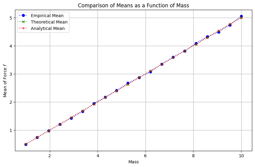
plt.plot(mass_values, empirical_means, label='Empirical Mean', linestyle=':', marker='o', color='blue')
plt.plot(mass_values, theoretical_means, label='Theoretical Mean', linestyle=':', marker='x', color='green')
plt.plot(mass_values, analytical_means, label='Analytical Mean', linestyle=':', marker='+', color='red')

plt.title('Comparison of Means as a Function of Mass')
plt.xlabel('Mass')
plt.ylabel('Mean of Force $f$')
plt.legend()
plt.grid(True)
plt.show()